Download
1 / 35
350 likes | 559 Views
SEASONAL DYNAMIC FACTOR ANALYSIS AND BOOTSTRAP INFERENCE: APPLICATION TO ELECTRICITY MARKET FORECASTING Carolina García-Martos, María Jesús Sánchez (Universidad Politécnica de Madrid) Julio Rodríguez (Universidad Autónoma de Madrid) Andrés M. Alonso (Universidad Carlos III de Madrid).

E N D
SEASONAL DYNAMIC FACTOR ANALYSIS AND BOOTSTRAP INFERENCE: APPLICATION TO ELECTRICITY MARKET FORECASTING Carolina García-Martos, María Jesús Sánchez (Universidad Politécnica de Madrid) Julio Rodríguez (Universidad Autónoma de Madrid) Andrés M. Alonso (Universidad Carlos III de Madrid)
OUTLINE 1. Objectives and motivation 2. Methodology: Previous results 3. Seasonal Dynamic Factor Analysis (SeaDFA). 4. Bootstrap scheme for SeaDFA 5. Simulation results 6. Application: Forecasting electricity prices in the Spanish Market 7. Conclusions
Objectives METHODOLOGY Extend nonstationary dynamic factor analysis to be able to reduce dimensionality in vector of time series with seasonality. Common factors follow a multiplicative VARIMA model. Inference for the parameters of the model by means of bootstrap techniques. APPLICATION Long-run forecasting of electricity prices in the Spanish market
2. Methodology. Previous results. • García-Martos, C., Rodríguez, J. and Sánchez, M.J. (2007). Mixed model for short-run forecasting of electricity prices: Application for the Spanish market, IEEE Transactions on Power Systems. • VARMA models for the 24 hours vector. Curse of dimensionality. • Alonso, A.M., Peña, D. and Rodríguez, J. (2008). A methodology for population projections: An application to Spain. • Take advantage of the common dynamics of the 24 hourly time series of electricity prices.
2. Methodology of de DFA. Antecedents and previous results. Dimensionality reduction Peña-Box Model (1987). Valid only for the stationary case. Lee-Carter Model (1992). Demographic application. Peña-Poncela Model (2004, 2006): Non-stationary Dynamic Factor Analysis. A priori test for the number of non-stationary and stationary factors. Alonso, A.M., García-Martos, C., Rodríguez, J. and Sánchez, M.J. (2008, working paper): Extension to the case in which common factors follow a multiplicative seasonal VARIMA model. Bootstrap procedure to make inference on parameters of the SeaDFA.
3. Seasonal Dynamic Factor Analysis (SeaDFA). Methodology:Use Dynamic Factor Analysis to extract common dynamics of the vector of time series. Particular case in which the vector of time series comes from a series with double seasonality. Common and specific component of seasonality.
3. Seasonal Dynamic Factor Analysis (SeaDFA). ytvector of m time series, generated by set of r common unobserved factors. ft is a vector of time series containing the r common factors. Ωloading matrix that relates the vector of observed series yt ,with the set of unobserved common factors. εtvector of specific components, m-dimensional, with zero mean and diagonal variance-covariance matrix. Common unobserved factors, ft, follow a multiplicative VARIMA model: (1-Bs)Ds(1-B)d ftφ(B) Φ(Bs) = c +θ(B)Θ(Bs)ut
3. Seasonal Dynamic Factor Analysis (SeaDFA). Measurement and transition equations in the state-space: State-space formulation is the natural way of writing down SeaDFA, which relates a m-dimensional vector of observed time series with an r-dimensional vector of unobserved common factors that follow a multiplicative seasonal VARIMA model.
j=1 Initialize procedure Kalman filter and smoother Log-likelihood LY(Θ) j = j+1 No Convergence Yes 3. Seasonal Dynamic Factor Analysis (SeaDFA). Estimation of the model is performed by EM algorithm. E-step M-step. Obtain Q, S, Ω, Φ, μ0, P00 END
3. Seasonal Dynamic Factor Analysis (SeaDFA). Estimation of the model is performed by EM algorithm. The expression for the log-likelihood of complete data is:
3. Seasonal Dynamic Factor Analysis (SeaDFA). EM ALGORITHM E-step Conditional expectation of log-likelihood:
3. Seasonal Dynamic Factor Analysis (SeaDFA). Where… … are obtained from the Kalman filter and smoother
3. Seasonal Dynamic Factor Analysis (SeaDFA). EM ALGORITHM M-step Maximization of the conditional expection of log-likelihood (E-step). Non-linear optimization procedure with non-linear constraints. Non linear restrictions appear between parameters involved in the seasonal multiplicative VARIMA model, i.e., between elements in .
4. Bootstrap scheme for SeaDFA 4.1 Estimate SeaDFA, parameters involved are obtained: 4.2 The specific factors are calculated: Here is important to introduce a correction for matrix estimation using the following relation: where can be expressed by the estimated loads and the variance of the state variables.
4. Bootstrap scheme for SeaDFA 4.3 Draw B resamples from the empirical distribution function of the centered and corrected specific factors: 4.4 Calculate the residuals and correct them in the same way that it was done for , but bearing in mind that we impose , so: 4.5 Draw B resamples from the empirical distribution function of the standarized residuals of the VARIMA model for the common factors.
4. Bootstrap scheme for SeaDFA 4.6 Generate B bootstrap replicas of the common factors using the transition equation: 4.7 Generate B bootstrap replicates of the SeaDFM using the bootstrap replicas of the common and specific factors obtained in steps 4.3 and 4.6:
4. Bootstrap scheme for SeaDFA From estimating the SeaDFA for each one of the B replicas obtained in step 4.7, we obtain the estimated bootstrap distribution functions of: Inference is based on percentiles obtained from the bootstrap distribution functions of the parameters involved.
4. Bootstrap scheme for forecasting Bootstrap procedure described is modified to replicate the conditional distribution of future observations given the observed vector of time series. For each specific and common factor the corresponding last observations are fixed. and the future bootstrap observation are generated by
5. Simulation results Bootstrap procedure was validated using a Monte Carlo experiment using three different models: Model 1: A common nonstationary factor (1-B)ft = c + wt, i.e. an I(1) with non null drift (c=3), for m=4 observed series. This model has been selected because it appears in Peña and Poncela (2004), and we have added the constant to validate its estimation, since we have included this possibility in our model. Model 2: A common nonstationary factor (1-B)(1-0.5B) ft = wt, for m=3 observed series. Model 3: We check the performance of our procedure when there is a seasonal pattern. There is a common nonstationary factor following a seasonal multiplicative ARIMA model (1-B7)(1-0.4B)(1-0.15B7)ft = wt, for m=4 observed series.
6. Application: Forecasting electricity prices in the Spanish Market Long-run forecasting in the Spanish market. Compute forecasts for year 2004 using data from January 1998 to December 2003.
6. Application: Forecasting electricity prices in the Spanish Market VARIMA(1,0,0)x(1,1,0)7 model with constant for the common factors.
6. Application: Forecasting electricity prices in the Spanish Market Inference using the bootstrap scheme described implies that Constants are not significant. The model is re-estimated including these constraints.
6. Application: Forecasting electricity prices in the Spanish Market Inference using the bootstrap scheme described implies that Φ121 not significant. The model is re-estimated including this constraint.
6. Application: Forecasting electricity prices in the Spanish Market Estimated loading matrix:
6. Application: Forecasting electricity prices in the Spanish Market
6. Application: Forecasting electricity prices in the Spanish Market Forecasts for the whole year 2004, using data from 1998-2003. Forecasting horizon varying from 1 day up to 1 year. MAPE for the whole year is 21.56%. Relationship with short-run forecasting MAPE (one-day-ahead). MAPE is around 13-15%. The mixed model of García-Martos et al (2007) obtained a short-run forecasting MAPE equal to 12.61%.
6. Application: Forecasting electricity prices in the Spanish Market MAPE for the whole year is 21.56% with SeaDFM and 45.62% with the Mixed Model.
6. Application: Forecasting electricity prices in the Spanish Market Third week of February 2004, MAPE 16.38%.
6. Application: Forecasting electricity prices in the Spanish Market 24th-30th May 2004, prediction intervals including uncertainty due to parameter estimation
6. Application: Forecasting electricity prices in the Spanish Market 20th-26th December 2004, prediction intervals including uncertainty due to parameter estimation
7. Conclusions Extension of the Non-Stationary Dynamic Factor Model to the case in which the common factors follow a multiplicative VARIMA model with constant. Constant included by means of an exogenous variable. Extension to the case in which there are exogenous variables in the SeaDFA is straightforward. Bootstrap procedure to make inference and forecasting. Valid for all models that can be expressed under state-space formulation. MAPE around 20% for year ahead forecasts of electricity prices. Most previous works obtain around 13% for one-day-ahead forecasts.
SEASONAL DYNAMIC FACTOR ANALYSIS AND BOOTSTRAP INFERENCE: APPLICATION TO ELECTRICITY MARKET FORECASTING Carolina García-Martos, María Jesús Sánchez (Universidad Politécnica de Madrid) Julio Rodríguez (Universidad Autónoma de Madrid) Andrés M. Alonso (Universidad Carlos III de Madrid)