Download
1 / 23
230 likes | 251 Views
Explore water vapor fluctuations within the convective boundary layer using large eddy simulations and observations from June 14, 2002. Discuss methodology, data scales, simulation comparisons, and insights on cloud formation.

E N D
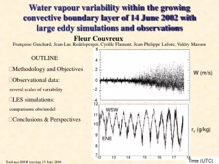
12 13 14 15 16 17 18 Water vapour variability within the growing convective boundary layer of 14 June 2002 with large eddy simulations and observations Fleur Couvreux Françoise Guichard, Jean-Luc Redelsperger, Cyrille Flamant, Jean-Philippe Lafore, Valéry Masson 6 OUTLINE • Methodology and Objectives • Observational data: several scales of variability • LES simulations: comparisons obs/model • Conclusions & Perspectives 4 2 W (m/s) 0 -2 -4 12 WSW 11 10 rv (g/kg) 9 ENE 8 7 Time (UTC)
IHOP observations: What are the fluctuations of water vapour mixing ratio observed within the growing convective boundary layer? 14 june 2002: BLE case What are the scales involved ? Is this day typical? • first goal : from observations and simulations, to explain the mecanisms responsible for the water vapour variability • second goal: to understand the role of such variability on cloud formation and maintenance Methodology & Objectives • LES : Is such a high resolution model able to represent the observed water vapour variability ?
A classic convective BL growth … but with large fluctuations of rv 2 Boundary layer mean value of & rv Early afternoon Zi (km) Time 12h 13h 14h 15h 16h 17h 18h 19h 1 2 Time 12h 13h 14h 15h 16h 17h 18h 19h Zi (km) morning 0 1 (K) 294 306 300 0 7 rv (g/kg) 10 12 Time in UTC=local time+5h
Data : • Soundings (35) • Lidars (DLR-DIAL, LEANDRE et SRL) • In-situ aircraft data (NRL-P3 et UWKA) • Surface flux measurements (ISSF) The 14 june 2002 case • Main characteristics : • « Relatively » simple case of a growing boundary layer: a well mixed boundary • layer reaching 1.5 km • High Pressure system, homogeneous temperature field • Weak subsidence constant whole day • Low shear and weak wind (< 5m/s) from N to NE • Existence of thermals (cf Cloud radar) • Small cumuli developed after 1500 UTC • NE/SW moisture gradient • Heavy precipitation the day before, coherent • distribution with moisture gradient
Soundings : Different variability at different scales Soundings in a 200 km wide domain 1700 UTC 1130 UTC rv rv 5 g/kg 3 g/kg Different scales of variability: evidence in soundings 2 soundings separated from less than 10 km rv 1830 UTC 1g.kg-1
rv measured by the DLR lidar 1500 1500 1500 W E 1000 1000 1000 Height (m) Height (m) Height (m) 500 500 500 ENE WSW Different scales of variability : aircraft data and lidars 12 Aircraft rv measurement 7 12 rv 8 1710 Time (UTC) 1745 12 rv + +0.7 3g.kg-1 8 1710 Time (UTC) 1.5 g.kg-1 rv’ -0.7 1710 Time (UTC) 1745
Initial profile observations rv Modelling: LES with Méso-NH (Lafore et al. 1998) • Simulation : • x=y=100m, z streched (< 50m in BL) • 3D turbulence scheme (Cuxart et al. 2000) • early morning to early afternoon (duration 7h) • a ‘realistic’ simulation: • ISFF2 surface fluxes (prescribed) homogeneous • initial sounding = composite of soundings at 1130 UTC • large scale advection estimated from MM5 simulations and soundings
Comparison obs/LES at 1800 UTC rv Mean profiles Temporal evolution of mean profiles rv
Time variations of boundary layer characteristics zi Sensitivity to surface fluxes : +Bo -> +zi Sensitivity to large-scale advection : +ADV -> +zi +Bo -> +m +Bo -> + qm Cf Bo ie SSH et SLH +ADV -> + m +ADV -> + qm Several factors : Ws -> zi ->, q Adv -> -> zi Adv q -> q … rv Validated reference simulation, quantification of sensibility to different forcings
Horizontal cross sections 11 11 11 5 5 5 10 10 10 3 3 3 9 9 9 8 8 8 1 1 1 7 7 7 6 6 6 -1 -1 -1 5 5 5 -3 -3 -3 v (K) W (m/s) rv (g/kg) 306 305.5 Z/zi=1. Z/zi=1. 305 10 km 304.5 304. 303.5 305 304.5 Z/zi=0.8 Z/zi=0.8 304. 303.5 305 304.5 Z/zi=0.3 Z/zi=0.3 304. 303.5
Characteristic length scale C()= Reference simulation at 17h Los from Lohou et al. (2002) Rv v w z/zi (m) rv length scale is larger than length scale of v, , w
rv-rv rv LEANDRE and LES horizontal cross-sections Measurements from LEANDRE LES Simulations 1.2 3.5 1.2 3.5 1.2 3.5 1.2 3.5 ~10 km ~10 km At 1600 UTC
5.5 5.5 6 6 6.5 6.5 7 7 7.5 7.5 8 8 8.5 8.5 9 9 9.5 9.5 10 10 10.5 10.5 Vertical cross sections LES rv & w DLR-DIAL rv Evidence of dry downdrafts Several thermals in one humid zone
Dry downdraft Overshooting updrafts zi Evaluation of histograms of , rv, w Z=0.4zi KA aircraft P3 aircraft model … max --- min w’ ’ Equivalent gaussian rv’
Second order moments 3 lidar 10km-long Cross-section at 1730 UTC LES 1700 & 1800 UTC __ simulation __ lidar DIAL o P3 o KA Strong relation between The inversion strength and the variance q à zi (g.kg-1) Max(rv) (g.kg-1) 1.2 0.72 0.81 0.41 0.56 5.7 MNH 4.4 MNH 4.3 DIAL 3.9 DIAL 4.1 DIAL rv
Joint probability distribution At z/zi=0.8 At z/zi=0.3 + z/zi + larger spectrum of w+ and q-
Conclusions: • Observations from 14 juin 2002 during IHOP_2002 : Several scales of variability ( < 10 km et > 10 km) • Evaluation of the LES Able to represent the variability observed at scales lower than 10 km (comparisons to soundings, lidars (DIAL et SRL), aircraft time-series) Quantification the impact of scales > 10 km on variability at scales < 10km • At first order, the boundary layer dynamics explain the observed variability at scales lower than 10 km even without surface heterogeneities and variability in the initial atmospheric state • Dry narrow downdrafts as a signature of the BL growth (via dynamics at the top) [Crum et al. (1987) and Weckwerth et al. (1996)] • impact on length scale, skewness, vertical transport.. • Negative skewness is common (cf other IHOP days)
Perspectives: • Systematic analysis of IHOP data : - objective : to identify pertinent parameters controlling the water vapour variability in the boundary layer (such as strength of inversion (,q), fluxes…) from more idealised simulations -> 1D parameterizations • Quantify time scales concerned by mechanisms involved in the water vapour variability: dry intrusion life time, transient state • Understand the impact of such a variability on cloud formation and maintenance
Development of the CBL (courtesy of Bart Geerts) 1330 UTC 1415 UTC 1530 UTC 1630 UTC 1730 UTC aspect ratio: 1:1
Surface fluxes Sensible heat flux Bo~1. Bo~0.5 Latent heat flux
Large scale forcings (advection) Horizontal advection of Horizontal advection of rv Large-scale forcings Deduced from MM5 Subsiding w