Download
1 / 18
180 likes | 465 Views
Chapter 5 Sampling Distribution of the Proportion. Estimation Proportion Sampling Proportion Law of Large Numbers Normal Approximation of Sample Proportion Estimating Sample Proportion. Estimation. Population/Target Population. Sample.

E N D
Chapter 5 Sampling Distribution of the Proportion Estimation Proportion Sampling Proportion Law of Large Numbers Normal Approximation of Sample Proportion Estimating Sample Proportion
Estimation Population/Target Population Sample In making generalizations about the population, we use our sample. For example if we want to know the mean GPA of WMU students, the sample mean is used.
Estimation In the GPA example, sample mean is used to estimate the population mean µ. Here, population mean µ is called a parameter. ParameterEstimate µ (population mean) (sample mean) σ (population SD) SD (sample SD) P (population proportion) (sample proportion)
Proportion Suppose TV World sells 60 extended warranties with 300 TV sets sold. The warranty sales rate is 60/300 = 0.20. If X is the number of TV sets sold with warranty (success) , then X is a binomial variable. When X is a binomial random variable with parameters n and p, it follows that the proportion of success in the sample is also random. In our example, 60/300=0.20 is the proportion of TV sets sold with warranty and n=300 is the sample size.
Sample Proportion = X/n = (number of successes)/ (total number of observations in the sample) In a binomial case, expected value is np give or take For sample proportion, is expected to be p give or take
Sampling Proportion From the TV world example, the proportion is expected to be : give or take
iClicker Recently, a random sample of 40 small retail businesses found that 32 had experienced cash flow problems in their first year of operation. By how much will we miss the true population proportion? a. 0.004 b. 0.0001 c. 0.2715 d. 0.0632 e. 0.80
Law of Large Numbers The sample proportion tends to get closer to the true population proportion as sample size increases. From the TV world example, if n is increased to 1200 and = 0.20, then The amount of miss (SE) of the sample proportion decreases.
Normal Approximation of Sample Proportion The distribution of is approximately normal with mean p and standard deviation In calculator, normalcdf(a,b, , )
Example If TV World sold 100 TV sets last year, the percentage of set sold with extended warranties is expected to be around 20% give or take 4%. Estimate the likelihood that the sold warranties with each TV is more than 25% of those sets, in other words, P[ > 0.25] P[ > 0.25] = normalcdf(0.25,99,0.20, ) = 0.1056
Example • From a random sample of 40 students, 6 responded that they are planning to go to graduate school. Calculate an estimate for p and the corresponding standard error.
Example What is the likelihood that less than 15% of the students will go to graduate school? P( ≤ .15 ) = normalcdf(-9999, .15, .15, ) = 0.5 What is the likelihood that 30% to 70% of the students will go to graduate school? P( .30≤ ≤ .70 ) = normalcdf(.30, .70, .15, ) = 0.004
Estimating Sample Proportion is an estimate of the population proportion We will miss it by the standard error of the proportion
Exercise 1. According to Horseman’s quarterly, 3 out of 5 racehorse lose money. A racing partnership has 49 horses in its stables. What is the probability that more than two-thirds of the stable’s horses will lose money?
Solution P( p ≥ 2/3 ) = normalcdf(2/3,99, .60, 0.0699854212) = 0.1704 The probability that more than 2/3 of the stable’s horses will lose money is 0.1704.
Exercise • 5. Historically, 92% of the overnight deliveries of a parcel service arrive the next morning before noon (considered “noon time” delivery). Suppose 300 deliveries are randomly selected for the purposes of the quality control. • What is the probability that more than 90% of the deliveries were on time? • What is the probability that less than 85% of the deliveries were on time?
Solution a. P( p ≥ 90% ) = normalcdf(.90,9999, .92, 0.0156631202) = 0.8992 The probability that more than 90% of the delivery is on time is 0.8992. b. P( p ≤ 85% ) = normalcdf(-9999,.85, .92, 0.0156631202) = 3.93E-6 = 0.00000393 The probability that less than 85% of the delivery is on time is 0.00000393.