Download
1 / 23
230 likes | 281 Views
Explore the connection between definite and indefinite integrals, marginal cost analysis, and numeric integration. Learn to evaluate definite integrals using antiderivatives and substitution techniques with real-world examples.

E N D
Chapter 5Integration Section 5 The Fundamental Theorem Of Calculus
Introduction to the Fundamental Theorem of Calculus The definite integral of a function f on an interval [a, b] is a number corresponding to the area between the graph of f and the x axis from x = a to x = b. The indefinite integral of a function is a family of antiderivatives. This section outlines the connection between these two integrals.
Introduction to the Fundamental Theorem of Calculus Suppose the daily cost function for a manufacturing firm is C(x) = 180x + 200 0 <x< 20. The graph shows the cost function, C(x).
Introduction to the Fundamental Theorem of Calculus • The marginal cost is C´(x) = 180 with graph shown. • The change in the cost as production increases from 5 units to 10 units is • C(10) – C(5) = • (180·10+200) – (180·5 + 200) • = 180(10 – 5) = $900 • The increase in cost corresponds to the area of the shaded region under the marginal cost function from x = 5 to x = 10.
Introduction to the Fundamental Theorem of Calculus • The change in cost from x = 5 to x = 10 is equal to the area between the marginal cost function and the x axis from x = 5 to x = 10.
Example 1 Comparing Change in Cost to Area under Marginal Cost Suppose a company has a cost function, C(x) = –7.5x2 + 305x + 625. (A) Graph C(x) for 0 <x< 20. Calculate the change in cost from x = 5 to x = 10, and indicate that change in cost on the graph. • Solution (A) The graph is shown with the change of cost $962.50 shown on the graph.
Example 1 Comparing Change in Cost to Area under Marginal Cost Suppose a company has a cost function, C(x) = –7.5x2 + 305x + 625. (B) Graph the marginal cost function, C´(x) for 0 <x< 20. Use a geometric formula to calculate the area between C´(x) and the x axis from x = 5 to x = 10. • Solution (B) C´(x) = –15x + 305. • The graph is shown. • The shaded region is a trapezoid with area 962.50.
Example 1 Comparing Change in Cost to Area under Marginal Cost Suppose a company has a cost function, C(x) = –7.5x2 + 305x + 625 (C) Compare the results from parts A and B. • Solution (C) In part (A), the change in cost was found to be $962.50. • In part (B), the area bounded by the marginal cost function and the x axis between x = 5 and x = 10 was found to be 962.50. • The change in cost is the same as the area bounded by the marginal cost function from x = 5 to x = 10.
Evaluating Definite Integrals By the fundamental theorem, any definite integral of a function f can be evaluated whenever we can find an antiderivative F and evaluate F(b) – F(a) for the limits of integration a and b. Antiderivatives of a function f differ by at most a constant. When using the fundamental theorem to evaluate a definite integral, we generally choose the simplest antiderivative by letting the constant C = 0.
Example 2 Evaluating Definite Integrals Solution We find an antiderivative F(x) for
Example 3 Definite Integrals and Substitution Techniques Solution Let u = 2x + 4, then du = 2 dx and
Example 3 Definite Integrals and Substitution Techniques continued
Example 3 Definite Integrals and Substitution Techniques • Solution With u = 2x + 4, du = 2dx and when x = 0, u = 4 and x = 1 gives u = 6. Substituting u = 2x + 4 and du = 2dx and changing the limits of integration we have,
Example 3 Definite Integrals and Substitution Techniques continued The graph shows the result of a numerical calculator process for estimating this definite integral.
Example 4 Computing Cost from Rate of Change in Cost A management service found that maintenance costs (dollars per year) increased at a rate of M ´(x) = 90x2 + 5,000, where M(x) is the total accumulated cost of maintenance for x years. Write a definite integral that represents the total maintenance cost from the end of the second year to the end of the seventh year. Evaluate the integral.
Example 5 Numerical Integration on a Graphing Calculator Use a graphing calculator to estimate the value of the definite integral to three decimal places. Solution, the integrand does not have an elementary antiderivative so we are unable to use the fundamental theorem to evaluate this definite integral. We use a numerical integration process programmed into a graphing calculator.
Example 5 Numerical Integration on a Graphing Calculator continued Using the TI-84 Plus CE, the keystrokes for this process are The calculator result is
Example 5 Numerical Integration on a Graphing Calculator continued The result of using a graphical process for approximating this definite integral is shown.
Example 6 Average Value of a Function Find the average value of f(x) = 6x2 – 2x over the interval [–3, 2].
Example 7 Average Price Given the supply equation, p = S(x) = 10e0.05x, find the average price (in dollars) over the supply interval [25, 35].