Ising Model
These slides provide some background material on the Ising model that I found at http://www3.nd.edu/~mcbg/tutorials/2006/tutorial/ising.html The slides that you can download from there credit Professor Mark Alber and Ivan Gregoretti. (The website looks great! Lots of neat material there.).

Ising Model
E N D
Presentation Transcript
These slides provide some background material on the Ising model that I found at http://www3.nd.edu/~mcbg/tutorials/2006/tutorial/ising.htmlThe slides that you can download from there credit Professor Mark Alber and Ivan Gregoretti.(The website looks great! Lots of neat material there.)
Ising Model Dr. Ernst Ising May 10, 1900 – May 11, 1998
Magnetism • As electrons orbit around the nucleus, they create a magnetic field Paramagnetism – atoms have randomly oriented magnetic spins - magnetic moments of atoms cancel out, no net magnetism - many elements Ferromagnetism – parallel alignment of magnetic spins - Fe, Co, Ni only
What is the Ising Model • Created by Ernst Ising as a linear model of magnetic spins • A simulation of any phenomena where each point has one of two values and interacts with its nearest neighbors only • A magnetic spin can have a value of either 1 or -1 • Energy of a system is calculated using the Hamiltonian H = - K Σ si sJ - B Σ si • K is a constant • si is the spin, -1 or 1, of the ith particle • I and J are adjacent particles • B is the magnitude of the externally applied magnetic field William Rowan Hamilton, 1805-1865
the idea behind a Monte Carlo simulation • Many systems cannot be described by equations • Many equations can not be solved • We forget about finding a solution and compile all the possible solutions and determine their probabilities • We take the solution of the highest probability • This works for systems with many individual components, because on average, they will all behave like the solution of the largest probability • We are interested in the average behavior, the most common behavior, because that’s what is predictable or controllable • Monte Carlo methods are statistical methods to find solutions of high probability
Metropolis Algorithm • One of Monte Carlo methods to arrive at a stable solution • Start with a random initial configuration • Suggest a change with probability p • Accept the change with probability q • Generate a random number from a random number generator of uniform distribution between 0 and 1 • Let the action be carried out if the random number generated < probability of action • Reiterate process starting again by suggesting a change
Important Features • Accepting higher energy configurations • Most accepted changes lead to lower energy configurations, but not all! • Higher energy configurations are accepted, although the probability is lower. • Important because if no higher energy configurations are accepted, the solution may get trapped in a local minimum of energy, unable to reach the global minimum • Ergodicity • Probability of reaching any configuration from any other must be > 0 • Initial condition is random and it must be able to reach the solution which is unknown, so it must be able to reach every other possible configuration
An Overview of the Program • Sets up a 1-D lattice of n points • Each point in the lattice is randomly assigned a value of 1 or -1 • Calculates the energy of the system according to the Hamiltonian H = - K Σ si sJ - B Σ siWhere J=1 , B=0 • Periodic boundary conditions - sn+1 = s1 - the system becomes a circle • Picks a random point and switches its magnetic moment • Calculates the energy of the configuration
…program overview • Compares energy of the system with and without the change • If the energy of the perturbed system is lower, the change is accepted with probability = 1 • If the energy of the perturbed system is higher, the change is accepted with probability = exp (-D/ k T) • Iterations of the routine lead to a configuration of global minimum of energy
The change is accepted with probability = exp (-D/ k T) • D= E2- E1 E1 = energy of current configuration E2 = energy of perturbed configuration (change in energy from current configuration to perturbed configuration) • k = 1.3806503*10^-23, Boltzmann’s constant • T = temperature (K) • Since E2 is bigger than E1, D is positive, k and T are also positive by nature • e is raised to a negative quantity; the expression will always yield a value between 0 and 1
Where this probability comes from: 1902 - Gibbs derived that the expression for the probability of an equilibrium configuration • P i = 1/Z exp(-E i / kT) • Z = Σi exp( – E i / kT ) • Z • the partition function • the normalizing constant, sum of all probabilities for all possible configurations. • Most times, a near impossibility to calculate • Due to the way nature works, a system changes in small steps and does not go very far from the thermal equilibrium situation. Taking advantage of this, we will create a random change and then compare the probability of either configuration as a thermal equilibrium configuration. • P1= 1/Z exp(-E1/ kT) • P2= 1/Z exp(-E2/ kT) • P = P2/P1 = exp((E1-E2) / kT) Josiah Willard Gibbs, 1839-1903
Markov Chain • The current situation depends only on the situation one time step before it • If the day is one time unit and weather is a Markov process, tomorrow's weather depends only on today’s weather. Prior days have no influence. • The Ising model is a Markov process. Andrei Andreyevich Markov 1856-1922
Ways of collecting data in the program • Plot energy of each point in the lattice at a given instant • Plot energy of system vs. time • Plot energy at steady state vs. temperature • Plot number of clusters at steady state vs. time
Left: A possible Ising Configuration Right: Energy vs. lattice point for the configuration on the left
Observations • At low temperatures • clusters form, alignment of spins • low entropy • low energy • At high temperatures • more randomness • high entropy • high energy • How come ?!
Mathematically probability = exp (-D/ k T) • At low temperatures, probability of accepting a higher energy change is low • At high temperatures, probability of accepting a higher energy change is higher
Scientifically Competing factors: Energy and Entropy • Entropy, S = a measure of disorder • Total energy, U • Free energy = energy available to do work • Helmoltz free energy, A A = U – TS , T = Temperature ~ Most stable system has lowest possible free energy ~ 2nd law of thermodynamics: Total entropy must stay constant or increase ~ Heat energy, example of disordered energy
Dr. Ernst Ising • - May 10, 1900 – born in Germany • 1924 – University of Hamburg, published his doctoral • thesis on linear chain of magnetic moments of 1 and -1, • and never returned to this research • He became a high school teacher • 1939 – Escaped Nazi Germany to Luxembourg • 1940 – Germany invaded Luxembourg • 1947 – Ising came to USA and became a teacher of physics and mathematics at State Teachers College in Minot, North Dakota • 1948 – became a physics professor at Bradley University, Illinois • 1949 – He found out his doctoral thesis had become famous • 1976 – retired from Bradley University • May 11, 1998 – He passed away.
The Ising Model~ 800 papers per year are published that use the Ising model~ areas of social behavior, neural networks, protein folding~ between 1969-1997, more than 12,000 papers published that use the Ising model
References • “Andrei Andreyevich Markov.” <http://www-history.mcs.st-andrews.ac.uk/Mathematicians/Markov.html> July 11, 2006. • Barkema, G.T. and M.E.J. Newman. Monte Carlo Methods in Statistical Physics. Clarendon Press, Oxford. 1999. • “Dr. Ernst Ising.” http://www.bradley.edu/las/phy/personnel/isingobit.html July 11, 2006. • “Ernst Ising and the Ising Model.” <http://www.physik.tu- dresden.de/itp/members/kobe/isingconf.html > July 11, 2006. • “Introduction to the Hrothgar Ising Model Unit.” <http://oscar.cacr.caltech.edu/Hrothgar/Ising/intro.html> July 11, 2006 • “Josiah Willard Gibbs.” <http://www-history.mcs.st-andrews.ac.uk/Mathematicians/Gibbs.html> July 11, 2006. • “Magnetism.” >http://www.materialkemi.lth.se/course_projects/HT- 2004/KK045/Magnetic%20Materials/MM%20final/magnetism.htm> July 11, 2006 • “Markov Chain.” Wikipedia. <http://en.wikipedia.org/wiki/Markov_chain> July 11, 2006. • “Sir William Rowan Hamilton.” http://www-history.mcs.st-andrews.ac.uk/Mathematicians/Hamilton.html July 11, 2006. • Weirzchon, S.T. “The Ising Model.” Wolfram Research. <http://scienceworld.wolfram.com/physics/IsingModel.html> July 11, 2006.
Acknowledgements Professor Mark Alber Ivan Gregoretti