Incorporating Small-Scale Effects into Large-Scale Solidification Models: Methodologies & Challenges
This study explores simple methods to incorporate small-scale effects into large-scale solidification models essential for understanding the casting processes, including dendrite growth and microsegregation phenomena. It emphasizes the need for advanced computational grids that resolve effects at different scales (from millimeters to nanometers). The integration of heat and mass transfer models with microsegregation predictions poses challenges but is vital for enhanced accuracy in simulating solidification. Through case studies, we also address the practical challenges of current computational technology and the implications for future modeling advancements.

Incorporating Small-Scale Effects into Large-Scale Solidification Models: Methodologies & Challenges
E N D
Presentation Transcript
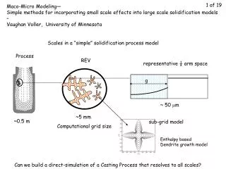
REV representative ½ arm space Process solid g ~ 50 mm ~5 mm sub-grid model ~0.5 m 1 of 19 Maco-Micro Modeling— Simple methods for incorporating small scale effects into large scale solidification models– Vaughan Voller, University of Minnesota Scales in a “simple” solidification process model Computational grid size Enthalpy based Dendrite growth model Can we build a direct-simulation of a Casting Process that resolves to all scales?
2 of 19 ~ 0.1 m chill A Casting The REV casting ~10 mm 103 101 10-1 10-3 10-5 10-7 10-9 Nucleation Sites heat and mass tran. equi-axed columnar grain formation The Grain Envelope growth ~ mm Time Scale (s) solute diffusion The Secondary Arm Space nucleation ~100 mm interface kinetics 10-9 10 10-3 10-1 Length Scale (m) The Tip Radius ~10 mm The Diffusive Interface f = 1 f = -1 ~1 nm Scales in Solidification Processes (after Dantzig) Can we build a direct-simulation of a Casting Process that resolves to all scales?
1 meter 6 decades 1 micron 3 of 19 Well As it happened not currently Possible 1000 20.6667 Year “Moore’s Law” 2055 for tip Voller and Porte-Agel, JCP 179, 698-703 (2002) Plotted The three largest MacWasp Grids (number of nodes) in each volume
~ 0.1 m chill A Casting The REV casting ~10 mm 103 101 10-1 10-3 10-5 10-7 10-9 Nucleation Sites heat and mass tran. equi-axed columnar grain formation The Grain Envelope growth ~ mm Time Scale (s) solute diffusion The Secondary Arm Space nucleation ~100 mm interface kinetics 10-9 10 10-3 10-1 Length Scale (m) The Tip Radius ~10 mm The Diffusive Interface f = 1 f = -1 ~1 nm 4 of 19 Scales in Solidification Processes (after Dantzig) To handle with current computational Technology require a “Micro-Macro” Model See Rappaz and co-workers Example a heat and Mass Transfer model Coupled with a Microsegregation Model
5 of 19 Solidification Modeling Process REV representative ½ arm space solid g sub-grid model ~ 50 mm Micro segregation—segregation and solute diffusion in arm space ~5 mm ~0.5 m Computational grid size from computation Of these values need to extract -- -- --
A C 6 of 19 Primary Solidification Solver g Transient mass balance g model of micro-segregation Iterative loop Cl T (will need under-relaxation) Give Liquid Concentrations equilibrium
Micro-segregation Model transient mass balance gives liquid concentration Solute Fourier No. Solute mass density after solidification Solute mass density before solidification Q -– back-diffusion Solute mass density of new solid (lever) 7 of 19 liquid concentration due to macro-segregation alone ½ Arm space of length l takes tf seconds to solidify In a small time step new solid forms with lever rule on concentration Need an easy to use approximation For back-diffusion
For special case Of Parabolic Solid Growth In Most other cases The Ohnaka approximation and And ad-hoc fit sets the factor Works very well 8 of 19 The parameter Model --- Clyne and Kurz, Ohnaka
Need to lag calculation one time step and ensure Q >0 m is sometimes take as a constant ~ 2 BUT In the time step model a variable value can be use Due to steeper profile at low liquid fraction ----- Propose 9 of 19 The Profile Model Wang and Beckermann
A model by Voller and Beckermann suggests If we assume that solid growth is close to parabolic m =2.33 in Parameter model In profile model 10 of 19 Arm-space will increase in dimension with time Coarsening This will dilute the concentration in the liquid fraction—can model be enhancing the back diffusion
11 of 19 Constant Cooling of Binary-Eutectic Alloy With Initial Concentration C0 = 1 and Eutectic Concentration Ceut = 5, No Macro segregation , k= 0.1 Use 200 time steps and equally increment 1 < Cl < 5 Calculating the transient value of g from Remaining Liquid when C =5 is Eutectic Fraction Parameter or Profile
Note Wide variation In Eutectic 12 of 19 Results are good across a range of conditions
13 of 19 Predictions of Eutectic Fraction With constant cooling Co = 4.9 Ceut = 33.2 k = 0.16 Comparison with Experiments Sarreal Abbaschian Met Trans 1986
14 of 19 Parabolic solid growth – No Second Phase – No Coarsening Use 10,000 equal of Dg C0 = 1, k = 0.13, a = 0.4 Use To calculate evolving segregation ratio
15 of 19 Performance of Models under parabolic growth no second phase in last liquid to solidify Prediction of segregation ratio (fit exponential through last two time points)
Solidification Solver 16 of 19 Calculate Transient solute balance in arm space predict T Predict g predict Cl Two Models For Back Diffusion Profile Parameter A A little more difficult to use Robust Easy to Use Poor Performance at very low liquid fraction— can be corrected With this Ad-hoc correction Excellent performance at all ranges Account for coarsening C My Method of Choice
Voller and Porte-Agel, JCP 179, 698-703 (2002) 1000 20.6667 Year “Moore’s Law” Model Directly 2055 for tip Tip-interface scale current for REV of 5mm (about 1018 nodes) 17 of 19 I Have a BIG Computer Why DO I need an REV and a sub grid model solid ~ 50 mm ~5mm (about 106 nodes) .5m
18 of 19 riser liquid Parameter Current estimate mushy empirical y solid chill Application – Inverse Segregation in a binary alloy Shrinkage sucks solute rich fluid toward chill – results in a region of +ve segregation at chill 100 mm Fixed temp chill results in a similarity solution
19 of 19 Comparison with Experiments Ferreira et al Met Trans 2004