Training Data

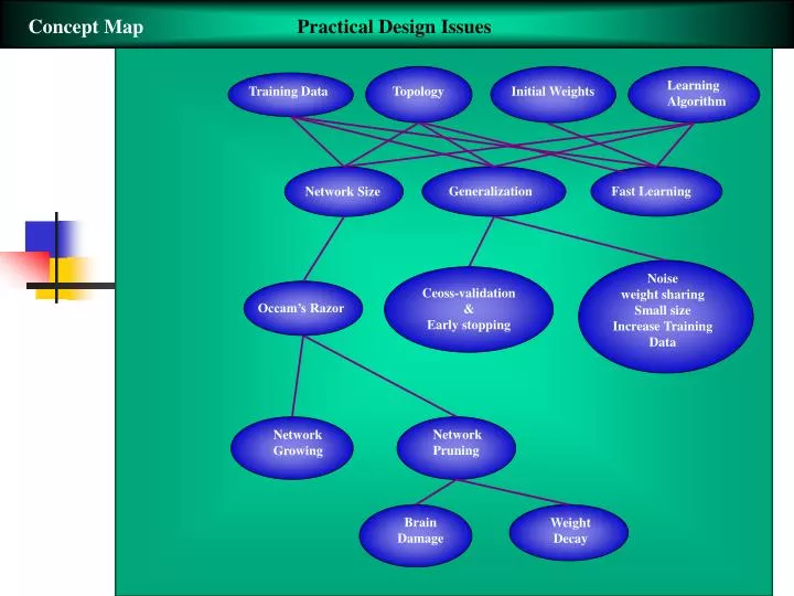
1. Concept Map Practical Design Issues Learning Algorithm Training Data Topology Initial Weights Generalization Fast Learning Network Size Noise weight sharing Small size Increase Training Data Ceoss-validation & Early stopping Occam’s Razor Network Pruning Network Growing Brain Damage Weight Decay

2. Chen & Mars Concept Map Fast Learning BP variants Cost Function Activation Function Training Data η No weight Learning For Correctly Classified Patterns Normalize Scale Present at Random Adaptive slope Momentum Architecture Other Minimization Method Fahlmann’s Modular Committee Conjugate Gradient

3. Chapter 4. Designing & Training MLPs • Practical Issues • Performance = f (training data, topology, initial weights, learning algorithm, . . .) • = Training Error, Net Size, Generalization. • How to prepare training data, test data ? • - The training set must contain enough info to learn the task. • - Eliminate redundancy, maybe by data clustering. • - Training Set size N > W/(N = # of training data, W = # of weights, • ε= Classification error permitted on Test data • Generalization error)

4. Ex. Modes of Preparing Training Data for Robot Control The importance of the training data for tracking performance can not be overemphasized. Basically, three modes of training data selection are considered here. In the regular mode, the training data are obtained by tessellating the robot’s workspace and taking the grid points as shown in the next page. However, for better generalization, a sufficient amount of random training set might be obtained by observing the light positions in response to uniformly random Cartesian commands to the robot. This is the random mode. The best generalization power is achieved by the semi-random mode which evenly tessellates the workspace into many cubes, and chooses a randomly selected training point within each cube. This mode is essentially a blend of the regular and the random modes.

5. Training Data Acquisition mode Random mode Regular mode Semi-random mode

6. Fig.10. Comparison of training errors and generalization errors for random and semi-random training methods.

7. Optimal Implementation • A. Network Size • Occam’s Razor : • Any learning machine should be • sufficiently large to solve a given problem, but not • larger. • A scientific model should favor simplicity or • shave off the fat in the model. • [Occam = 14th century British monk]

8. E E Number of Epochs a. Network Growing: Start with a few / add more (Ref. Kim, Modified Error BP Adding Neurons to Hidden Layer, J. of KIEE 92/4) If E > 1 and E < 2, Add a hidden node. Use the current weights for existing weights and small random values for newly added weights as initial weights for new learning. b. Network Pruning ① Remove unimportant connections After brain damage, retrain the network.  Improves generalization. ② Weight decay: after each epoch c. Size Reduction by Dim. Reduction or Sparse Connectivity in Input Layer [e.g. Use 4 random instead of 8 connections]

10. B. Generalization : Train (memorize) and Apply to an Actual problem (generalize) Poor Good test(O) test(O) train(X) train(X) Overfitting (due to too many traning samples, weights) noise R X T : Training Data X : Test Data R' T R : NN with Good Generalization R' : NN with Poor Generalization U

11. Learning Validation Test Set Subset Subset Training Set Mean- Square Validation Error sample Early Training stopping sample point 0 Number of epochs For good generalization, train with Learning Subset. Check on validation set. Determine best structure based on Validation Subset [10% at every 5-10 iterations]. Train further with the full Training Set. Evaluate on test set. Statistics of training (validation) data must be similar to that of test (actual problem) data. Tradeoff between training error and generalization ! Stopping Criterion Classification : Stop upon no error Function Approximation : check

12. An Example showing how to prepare the various data sets to learn an unknown function from data samples

13. Other measures to improve generalization. • Add Noise (1-5 %) tothe Training Data or Weights. • Hard (Soft) Weight Sharing (Using Equal Values for Groups of Weights) • Can Improve Generalization. • For fixed training data, the smaller the net the better the generalization. • Increase the training set to improve generalization. • For insufficient training data, use leave-one (some)-out method • = Select an example and train the net without this example, evaluate with this unused example. • If still does not generalize well, retrain with the new problem data. • C. Speeding Up [Accelerating] Convergence • - Ref. Book by Hertz, AI Expert Magazine 91/7 • To speed up calculation itself: • Reduce # Floating Point Ops by Using a Fixed Point Arithmetic • And Use a Piecewise-Linear approximation for the sigmoid.

14. Students’ Questions from 2005 What will happen if more than 5-10 % validation data are used ? Consider 2 industrial assembly robots for precision jobs made by the same company with an identical spec. If the same NN is used for both, then the robots will act differently. Do we need better generalization methods to compensate for this difference ? Large N may increase noisy data. However, wouldn’t large N offset the problem by yielding more reliability ? How big an influence would noise have upon misguided learning ? Wonder what measures can prevent the local minimum traps.

15. Is there any mathematical validation for the existence of a stopping point in validation samples ? The number of hidden nodes are adjusted by a human. An NN is supposed to self-learn and therefore there must be a way to automatically adjust the number of the hidden nodes.

17. ①Normalize Inputs, Scale Outputs. Zero mean, Decorrelate (PCA) and Covariance equalization

18. ② Start with small uniform random initial weights [for tanh] : ③ Present training patterns in random (shuffled) order (or mix different classes). ④ Alternative Cost or Activation Functions Ex. Cost Use with as targets or ( , , at )

19. ⑤ Fahlman's Bias to Ensure Nonzero for output units only or for all units For output unitsonly -- drop . ⑥ Chen & Mars Differential step size Cf. Principe’s Book recommends . Best to try diff. values. ⑦ (Accelerating BP Algorithm through Omitting Redundant Learning, J. of KIEE 92/9 ) If , Ep < do not update weight on the pth training pattern – NO BP E p e p

20. ⑩ Plaut Rule ⑧ Ahalt - Modular Net ⑨ Ahalt - Adapt Slope (Sharpness) Parameters vary  in

21. Reason for Slow Convergence + with momentum without momentum ⑪ Jacobs - Learning Rate Adaptation [Ref. Neural Networks, Vol. 1, No. 4, 88. ] a. Momentum : In plateau, where is the effective learning rate

22. i t b. rule : where For actual parameters to be used, consult Jacob’s paper and also “Getting a fast break with Backprop”, Tveter, AI Expert Magazine, excerpt from pdf files that I provided.

23. Students’ Questions from 2005 Is there any way to design a spherical error surface for faster convergence ? Momentum provides inertia to jump over a small peak. Parameter Optimization technique seems to a good help to NN design. I am afraid that optimizing even the sigmoid slope and the learning rate may expedite overfitting. In what aspect is it more manageable to remove the mean, decorrelate, etc. ? How does using a bigger learning rate for the output layer help learning ? Does the solution always converge if we use the gradient descent ?

24. Are there any shortcomings in using fast learning algorithms ? In the Ahalt’s modular net, is it faster for a single output only or all the outputs than an MLP ? Various fast learning methods have been proposed. Which is the best one ? Is it problem-dependent ? The Jacobs method cannot find the global min. for an error surface like:

25. ⑫ Conjugate Gradient : Fletcher & Reeves Line Search If  is fixed and  Gradient Descent If  Steepest Descent

26. GradientDescent SteepestDescent ConjugateGradient Gradient D.+ Line Search Steepest Descent + Momentum SD GD w(n) w(n) w(n+1) w(n+1) = = w(n+2) w(n+2) Momentum CG w(n) w(n+1) w(n-1) w(n) s(n+1) w(n+1)

27. If : Conjugate Gradient 1) Line Search 2) Choose  such that From Polak-Ribiere Rule :

28. End START Initialize Line Search N Y Y N

29. Comparison of SD and CG Steepest Descent Conjugate Gradient Each step takes a line search. For N-variable quadratic functions, converges in N steps at most Recommended: Steepest Descent + n steps of Conjugate Gradient + Steepest Descent + n steps of Conjugate Gradient + 

30. X. Swarm Intelligence • What is “swarm intelligence” and why is it interesting? • Two kinds of swarm intelligence • particle swarm optimization • ant colony optimization • Some applications • Discussion

31. What is “Swarm intelligence”? I can’t do… • “Swarm Intelligence is a property of systems of non-intelligent agents exhibiting collectively intelligent behavior.” • Characteristics of a swarm • distributed, no central control or data source • no (explicit) model of the environment • perception of environment • ability to change environment We can do…

32. Group of friends each having a metal detector are on a treasure finding mission. Each can communicate the signal and current position to the n nearest neighbors. If you neighbor is closer to the treasure than him, you can move closer to that neighbor thereby improving your own chance of finding the treasure. Also, the treasure may be found more easily than if you were on your own. Individuals in a swarm interact to solve a global objective in a more efficient manner than one single individual could. A swarm is defined as a structured collection of interacting organisms [ants, bees, wasps, termites, fish in schools an birds in flocks] or agents. Within the swarms, individuals are simple in structure, but their collective behaviors can be quite complex. Hence, the global behavior of a swam emerges in a nonlinear manner from the behavior of the individuals in that swarm. The interaction among individuals plays a vital role in shaping the swarm’s behavior. Interaction aids in refining experiential knowledge about the environment, and enhances the progress of the swarm toward optimality. The interaction is determined genetically or throgh social interaction. Applications: function optimization, optimal route finding, scheduling, image and data analysis.

33. Why is it interesting? • Robust nature of animal problem-solving • simple creatures exhibit complex behavior • behavior modified by dynamic environment e.g.) ants, bees, birds, fishes, etc,.

34. Two kinds of Swarm intelligence • Particle swarm optimization • Proposed in 1995 by J. Kennedy and R. C. Eberhart • based on the behavior of bird flocks and fish schools • Ant colony optimization • defined in 1999 by Dorigo, Di Cargo and Gambardella • based on the behavior of ant colonies

35. 1. Particle Swarm Optimization • Population-based method • Has three main principles • a particle has a movement • this particle wants to go back to the best previously visited position • this particle tries to get to the position of the best positioned particles

36. Four types of neighborhood • star (global) : all particles are neighbors of all particles • ring (circle) : particles have a fixed number of neighbors K (usually 2) • wheel : only one particle is connected to all particles and act as “hub” • random : N random conections are made between the particles

38. algorithm Initialization : xid(0) = random value, vid(0) = 0; Calculate performance : F (xid(t)) = ? (F : performance) Update best particle : F (xid(t)) is better than the pbest -> pbest = F(xid(t)), pid = xid(t), Same for the gbest Move each particle : See next slide Until system converges

39. Particle Dynamics for convergence c1+ c2 < 4 [Kennedy 1998]

42. Examples http://uk.geocities.com/markcsinclair/pso.html http://www.engr.iupui.edu/~shi/PSO/AppletGUI.html

43. ⑬ Fuzzy control of Learning rate, Slope (Principe’s, Chap. 4.16) ⑭ Local Minimum Problem • Restart with different initial weights, learning rates, and number • of hidden nodes • Add (and anneal) noise a little (zero mean white Gaussian) to weights or training data [desired output or input (for better generalization) ] • Use {Simulated Annealing} or {Genetic Algorithm Optimization then BP} ⑮ Design aided by aGraphic User Interface– NN Oscilloscope Look at Internal weights/Node Activitieswith Color Coding

44. Students’ Questions from 2005 When the learning rate is optimized and initialized, there must be a rough boundary for it. Just an empirical way to do it ? In Conjugate Gradient, s(n) = -g(n+1) … The learning rate annealing just keeps on decreasing the error as n without looking at where in the error surface the current weights are. Is this OK ? Conjugate Gradient is similar to Momentum in that old search direction is utilized in determining the new search direction. It is also similar to rule using the past trend. Is CG always faster converging than the SD ? Do the diff. initial values of the weights affect the output results ? How can we choose them ?