Data science training.
Excelr offers Data Science Course Training and Certification in Hyderabad.It also provides business partner of Tata Consultancy Services(TCS) TCS will consider the successfull Excelr students for opportunities

Data science training.
E N D
Presentation Transcript
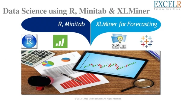
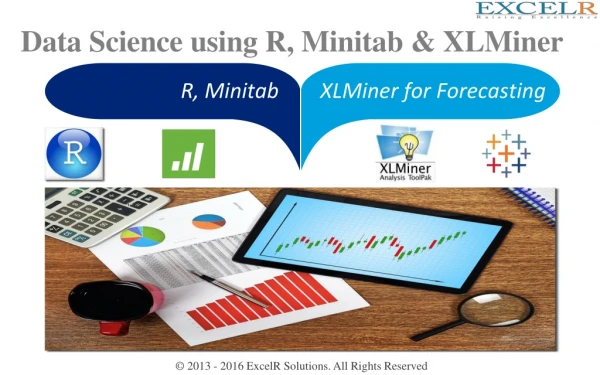
Data Science using R, Minitab & XLMiner R, Minitab XLMiner for Forecasting © 2013 - 2016 ExcelR Solutions. All Rights Reserved
My Introduction Name: Bharani Kumar Education: IIT Hyderabad Indian School of Business Professional certifications: PMP PMI-ACP PMI-RMP CSM LSSGB LSSBB SSMBB ITIL Agile PM Project Management Professional Agile Certified Practitioner Risk Management Professional Certified Scrum Master Lean Six Sigma Green Belt Lean Six Sigma Black Belt Six Sigma Master Black Belt Information Technology Infrastructure Library Dynamic System Development Methodology Atern © 2013 - 2016 ExcelR Solutions. All Rights Reserved
My Introduction 4 RESEARCH in ANALYTICS, DEEP LEARNING & IOT DATA SCIENTIST 3 2 Deloitte Driven using US policies 1 Infosys Driven using Indian policies under Large enterprises ITC Infotech Driven using Indian policies SME HSBC Driven using UK policies © 2013 - 2016 ExcelR Solutions. All Rights Reserved
Tuckman Model © 2013 - 2016 ExcelR Solutions. All Rights Reserved
AGENDA Data Mining – Supervised & Unsupervised (Machine Learning) Text Mining & NLP Data Visualization using Tableau AGENDA © 2013 - 2016 ExcelR Solutions. All Rights Reserved
What does it take to be a DATA SCIENTIST? Domain Knowledge All Agenda Topics Statistical Analysis Data Minin g Practice Data Visualizatio n Forecasting Successful Data Scientist © 2013 - 2016 ExcelR Solutions. All Rights Reserved
Welcome to the Information Age … … drowning in data and starving for Knowledge © 2013 - 2016 ExcelR Solutions. All Rights Reserved
BIG DATA! 500 million tweets every day, 1.3 billion accounts YouTube users upload 100 hours of video every minute 306 items are purchased every second 26.6 Million transactions per day 100 terabytes of data uploaded daily http://www.dnaindia.com/scitech/report-facebook-saw- one-billion-simultaneous-users-on-aug-24-2119428 Processing 100 petabytes a day (1 petabyte = 1000 terabytes) More than 1 million customer transactions every hour https://www.techinasia.com/alibaba-crushes-records-brings-143-billion-singles-day © 2013 - 2016 ExcelR Solutions. All Rights Reserved
Why Tableau? © 2013 - 2016 ExcelR Solutions. All Rights Reserved
Why Tableau? © 2013 - 2016 ExcelR Solutions. All Rights Reserved
Why Tableau? © 2013 - 2016 ExcelR Solutions. All Rights Reserved
Why Tableau? © 2013 - 2016 ExcelR Solutions. All Rights Reserved
Agenda – Basic Statistics Data Types – Continuous, Discrete, Nominal, Ordinal, Interval, Ratio, Random Variable, Probability, Probability Distribution 1 First, second, third & fourth moment business decisions 2 3 4 5 Graphical representation – Barplot, Histogram, Boxplot, Scatter diagram Simple Linear Regression Hypothesis Testing © 2013 - 2016 ExcelR Solutions. All Rights Reserved
Data Types – Continuous & Discrete © 2013 - 2016 ExcelR Solutions. All Rights Reserved
Data Types – Preliminaries © 2013 - 2016 ExcelR Solutions. All Rights Reserved
Random Variable © 2013 - 2016 ExcelR Solutions. All Rights Reserved
Probability © 2013 - 2016 ExcelR Solutions. All Rights Reserved
Probability Distribution © 2013 - 2016 ExcelR Solutions. All Rights Reserved
Probability Applications © 2013 - 2016 ExcelR Solutions. All Rights Reserved
Sampling Funnel Population Sampling Frame SRS Sample © 2013 - 2016 ExcelR Solutions. All Rights Reserved
Measures of Central Tendency Central Tendency Population Sample Mean / Average Median Middle value of the data Mode Most occurring value in the data “Every American should have above average income, and my Administration is going to see they get it.” – American President © 2013 - 2016 ExcelR Solutions. All Rights Reserved
Measures of Dispersion © 2013 - 2016 ExcelR Solutions. All Rights Reserved
Measures of Dispersion Dispersion Population Sample Variance Standard Deviation Range Max – Min © 2013 - 2016 ExcelR Solutions. All Rights Reserved
Expected Value For a probability distribution, the mean of the distribution is known as the expected value The expected value intuitively refers to what one would find if they repeated the experiment an infinite number of times and took the average of all of the outcomes Mathematically, it is calculated as the weighted average of each possible value The expected value for a discrete random variable X, denoted by μ, is: formula for calculating the The variance of a discrete random variable X, denoted by σ2 is © 2013 - 2016 ExcelR Solutions. All Rights Reserved
Graphical Techniques – Bar Chart © 2013 - 2016 ExcelR Solutions. All Rights Reserved
Graphical Techniques – Histogram A Histogram Represents the frequency distribution, i.e., how many observations take the value within a certain interval. © 2013 - 2016 ExcelR Solutions. All Rights Reserved
Skewness & Kurtosis Third and Fourth moments Skewness Kurtosis • • A measure of asymmetry in the distribution Mathematically it is given by E[(x-µ/σ)]3 Negative skewness implies mass of the distribution is concentrated on the right • A measure of the “Peakedness” of the distribution Mathematically it is given by E[(x-µ/σ)]4-3 For Symmetric distributions, negative kurtosis implies wider peak and thinner tails • • • © 2013 - 2016 ExcelR Solutions. All Rights Reserved
Graphical Techniques – Box Plot Range(IQR): The middle half of a data set falls within the inter- quartile range Inter- quartile Box Plot : This graph shows the distribution of data by dividing the data into four groups with the same number of data points in each group. The box contains the middle 50% of the data points and each of the two whiskers contain 25% of the data points. It displays two common measures of the variability or spread in a data set Range : It is represented distance between the smallest value and the largest value, including any outliers. If you ignore outliers, the range is illustrated by the distance between the opposite ends of the whiskers on a box plot by the © 2013 - 2016 ExcelR Solutions. All Rights Reserved
Normal Distribution The normal random variable takes values from -∞ to +∞ The Probability associated with any single value of a random variable is always zero Area under the entire curve is always equal to 1 © 2013 - 2016 ExcelR Solutions. All Rights Reserved
Normal Distribution Characterized by a bell shaped curve Has the following properties: 95.46% of the values lie within ±2 σ from the mean 99.73% of the values lie within ± 3σ from the mean 68.26% of values lie within ±1 σ from the mean © 2013 - 2016 ExcelR Solutions. All Rights Reserved
Normal Distribution Characterized by mean, µ, and standard deviation, σ X~N(µ,σ) © 2013 - 2016 ExcelR Solutions. All Rights Reserved
Z scores, Standard Normal Distribution • For every value (x) of the random variable X, we can calculate Z score: Z = X−µ σ • Interpretation − How many standard deviations away is the value from the mean ? © 2013 - 2016 ExcelR Solutions. All Rights Reserved
Calculating Probability from Z distribution Suppose GMAT scores can be reasonably modelled using a normal distribution − µ = 711 σ = 29 What is p(x ≤ 680)? Step 1: Calculate Z score corresponding to 680 - Z = (680-711)/29 = -1.06 Step 2: Calculate the probabilities using Z – Tables - P(Z ≤ -1) = 0.14 © 2013 - 2016 ExcelR Solutions. All Rights Reserved
Calculating Probability from Z distribution • What is P( 697 ≤ X ≤ 740) ? • Step 1 : Use P(x1 ≤ X ≤ x2) = Use P( X ≤ x2) − P( X ≤ x1) • Step 2 : Calculate P( X ≤ x2) and P( X ≤ x1) as before P( X ≤ 740) = P( Z ≤ 1) = 0.84 ; P( X ≤ 697) = P( Z ≤ - 0.5) = 0.31 • Step 3 : Calculate P( 697 ≤ X ≤ 740 ) = 0.84 – 0.31 = 0.53 © 2013 - 2016 ExcelR Solutions. All Rights Reserved
Normal Quantile (Q-Q) Plot Sample Quantiles Theoretical Quantiles © 2013 - 2016 ExcelR Solutions. All Rights Reserved
Sampling variation Sample mean varies from one sample to another Sample mean can be (and most likely is) different from the population mean Sample mean is a random variable © 2013 - 2016 ExcelR Solutions. All Rights Reserved
Central Limit Theorem The Distribution of the sample mean - will be normal when the distribution of data in the population is normal - will be approximately normal even if the distribution of data in the population is not normal if the “sample size” is fairly large _ Mean ( X ) = µ ( the same as the population mean of the raw data) Standard Deviation (X) = , where σ is the population standard deviation and n is the sample size σ √? - This is referred to as standard error of mean The standard error of the mean estimates the variability between samples whereas the standard deviation measures the variability within a single sample © 2013 - 2016 ExcelR Solutions. All Rights Reserved
Sample Size Calculation A Sample Size of 30 is considered large enough, but that may /may not be adequate More Precise conditions - n > 10( K3)2, where ( K3) is sample skewness and - n > 10( K4) , where ( K4) is sample kurtosis © 2013 - 2016 ExcelR Solutions. All Rights Reserved
Confidence Interval • What is the Probability of tomorrow’s temperature being 42 degrees ? Probability is ‘0’ • Can it be between [-50⁰C & 100⁰C] ? © 2013 - 2016 ExcelR Solutions. All Rights Reserved
Case Study: Confidence Interval • A University with 100,000 alumni is thinking of offering a new affinity credit card to its alumni. • Profitability of the card depends on the average balance maintained by the card holders. • A Market research campaign is launched, in which about 140 alumni accept the card in a pilot launch. • Average balance maintained by these is $1990 and the standard deviation is $2833. Assume that the population standard deviation is $2500 from previous launches. • What we can say about the average balance that will be held after a full−fledged market launch ? © 2013 - 2016 ExcelR Solutions. All Rights Reserved
Interval estimates of parameters • Based on sample data − The point estimate for mean balance = $1990 − Can we trust this estimate ? • What do you think will happen if we took another random sample of 140 alumni ? • Because of this uncertainty, we prefer to provide the estimate as an interval (range) and associate a level of confidence with it Interval Estimate = Point Estimate ± Margin of Error © 2013 - 2016 ExcelR Solutions. All Rights Reserved
Confidence Interval for the Population Mean Start by choosing a confidence level (1-α) % (e.g. 95%, 99%, 90%) Then, the population mean will be with in _ σ X ± Z1-ᾳ where Z1-ᾳsatisfies p( -Z1-ᾳ≤ Z ≤ Z1-ᾳ) = 1-ᾳ √? Interval Estimate = Point Estimate ± Margin of Error Margin of error depends on the underlying uncertainty, confidence level and sample size © 2013 - 2016 ExcelR Solutions. All Rights Reserved
Calculate Z value - 90%, 95% & 99% © 2013 - 2016 ExcelR Solutions. All Rights Reserved
Confidence Interval Calculation • Based on the survey and past data _ − n = 140; σ = $2500; X = $ 1990 − σX - σ √? 2500 √140 = = = 211.29 • Construct a 95% confidence interval for the mean card balance and interpret it ? • Construct a 90% confidence interval for the mean card balance and interpret it ? © 2013 - 2016 ExcelR Solutions. All Rights Reserved
Confidence Interval Interpretation Consider the 95% Confidence interval for the mean income : [$1576, $2404] Does this mean that - The mean balance of the population lies in the range ? - The mean balance is in this range 95% of the time ? - 95% of the alumni have balance in this range ? Interpretation 1 : Mean of the population has a 95% chance of being in this range for a random sample Interpretation 2 : Mean of the population will be in this range for 95% of the random samples © 2013 - 2016 ExcelR Solutions. All Rights Reserved
What if we don’t know Sigma? • Suppose that the alumni of this university are very different and hence population standard deviation from previous launches can not be used We replace σ with our best guess (point estimate) s, which is the standard deviation of the sample: Calculate • If the underlying population is normally distributed , T is a random variable distributed according to a t-distribution with n-1 degrees of freedom Tn-1 • Research has shown that the t-distribution is fairly robust to deviation of the population of the normal model © 2013 - 2016 ExcelR Solutions. All Rights Reserved
Student’s t-distribution As n tn ꝏ N(0,1) i.e., as the degrees of the freedom increase, the t-distribution approaches the standard normal distribution © 2013 - 2016 ExcelR Solutions. All Rights Reserved
Confidence Interval for mean with unknown Sigma © 2013 - 2016 ExcelR Solutions. All Rights Reserved
Calculating t-value • Construct a 95% confidence interval for the mean card balance and interpret it? _ − n = 140; σ = $2500; X = $ 1990 -=2833 − σX = 239.46 √140 Calculate t0.95, 139 = 1.98 Then the 95% confidence interval for balance is [$1516, $2464] © 2013 - 2016 ExcelR Solutions. All Rights Reserved
Hypothesis Testing H1 is TRUE Ho is TRUE Start with Hypothesis about a Population Parameter Right Decision Type II error Fail to Reject Ho Confidence 1-α Collect Sample Information Right Decision Type I error Power Reject Ho 1-β Reject/Do Not Reject Hypothesis The factors that affect the power of a test include sample size, effect size, population variability, and ?. Power and ? are related as increasing ? decreases ?. Since power is calculated by 1 minus ?, if you increase ?,You also increase the power of a test. The maximum power a test can have is 1, whereas the minimum value is 0. © 2013 - 2016 ExcelR Solutions. All Rights Reserved