Array Processors
Array Processors. Characteristics. A single control processor (CP) issues instructions to a multiple array of processing elements (PE) PE ’ s execute instructions in a lock-step mode. All processors execute the same instruction at any time (synchronous array processors)

Array Processors
E N D
Presentation Transcript
Characteristics • A single control processor (CP) issues instructions to a multiple array of processing elements (PE) • PE’s execute instructions in a lock-step mode. All processors execute the same instruction at any time (synchronous array processors) • Each processor operates on its own data stream. All processors are active simultaneously (data-parallel architectures) 5. The degree of parallelism depends on the number of PE’s available (hardware intensive architectures) • PE’s are interconnected by a data exchange network.
SIMD organization • Consider again the vector operation C = A + B which can be implemented by an array of N PE’s for N operations.
SIMD organization • Consider element by element the addition of two N-element vectors A and B to create the sum vector C. That is: C[i]=A[i]+B[i] 1≤ i ≤ N • As noted before, this computation requires N add times plus the loop control overhead on an SISD. Also, the SISD processor has to fetch the instructions corresponding to this program from memory each time through the loop.
SIMD organization • However this figure shows the SIMD implementation of this computation; using N PEs, which consists of multiple PEs, one CP, and the memory system: C[i]=A[i]+B[i] 1≤ i ≤ N Figure 5.1 here
SIMD organization • The elements-of arrays A and B are distributed over N memory blocks, and hence, each PE has access to one pair of operands to be added. Thus, the program for the SIMD consists of one instruction: C=A+B
SIMD organization • Therefore on a SIMD system the one instruction C=A+B is equivalent to, C[i]=A[i]+B[i] 1≤ i ≤ N • where i represents the PE that is performing the addition of the i elements, and the expression in parentheses implies that N PEs are active simultaneously.
SIMD organization • What is the execution time?
SIMD organization C[i]=A[i]+B[i] 1≤ i ≤ N • The execution time for the above computation is one addition time. No other overhead is needed. But data needs to be structured in N memory blocks to provide for the simultaneous access of the N data elements.
Memory • each PE is connected to its own memory block.
Memory • If memory addresses are interleaved, instructions of a program would spread among all memory blocks. Since the CP is fetching instructions from several blocks, a memory block can be assigned for programs to be accessed directly by the CP. Effects: actual memory partition between data and instructions, and size of programs are restricted.
Memory • The CP could also be configured with its own memory. • Note this means all of the PE memory is no longer available to the CP, this could place restrictions on the size of CP programs.
Memory • An n × n switch is another alternative this will allow each PE to access any memory block, and data structuring becomes more flexible. • To provide for simultaneous access data structuring is important. • Laying out the data so that conflicts occur results in inefficiencies even in an nxn structure.
Memory • Given efficient data layout what is the down side to an nxn switch arrangement?
Control Processor • fetches instructions and decodes them. • transfers A/L operations to the PE’s and generates controls signals for their execution • calculates addresses • it might retrieve common data from memory and broadcast it to all PE’s.
A/L Processors • respond to control signals from the CP to execute A/L operations.
Interconnection Network (IN) • memory-to-PE interconnection. Required to access data directly; An n × n switch provides this interconnection. • PE-to-PE interconnection. Required if data exchange between PE’s is needed.
IN • Type 1 SIMD
IN • Type 2
IN • Type 3
Performance Considerations • Consider the task of computing the column sum of an (N × N) matrix. The figure in the next slide shows the data structure used in an SIMD with N PEs. Each PE has access to one column of the matrix. Thus, the program shown in (b) can be used to perform the column sum computation. The column sum is computed by traversing the loop N times. Thus, the order of computation is N compared to N2 required on an SISD.
Performance Considerations • Fig 5.3
Performance Considerations • The assembly language equivalent of the program in (b) is shown in (c). In this program, instructions LDA, ADD, and STA are executed simultaneously by all the PEs while the instructions LDX, DEX, BNZ, and HLT are executed by the CP. Thus the instruction set of an SIMD is similar to that of an SISD except that the arithmetic/logic instructions are performed by multiple PEs simultaneously.
Performance Considerations • Consider a program that normalizes the columns in the previous data structure w.r.t the first element. (first element cannot be zero or else it’s skipped) • Therefore the columns associated with the 0 first element are deactivated during this program execution.
Performance Considerations • Consider the program segment depicted by the flowchart of figure in the next slide. Here, A, B, C, and D represent blocks of instructions. If this program were for an SISD, the processor, after executing A, either B or C will execute depending on the value of X and then would execute D. In an SIMD, some data streams satisfy X = 0 and the others satisfy X means that some PEs execute B and the others execute C and that all PEs eventually execute D.
Performance Considerations • Figure 5.4
IN • To accommodate this computation and to retain the instruction lock-step mode of operation, the branch operation is converted into a sequential operation as shown in (b). Note that all the PEs are not active during the execution of blocks C and B, and hence, the SIMD hardware is not being utilized efficiently. As such, for an SIMD to be efficient, conditional branches should be avoided as much as possible.
Memory Organization • Consider the popular matrix multiply algorithm for an SIMD depicted by the program in the next figure. • Here, to compute the element C[i, j], the ith row elements of A are multiplied element-by-element by the jth column elements of B and the products are accumulated. The algorithm executes in N3 time.
Memory Organization • Figure 5.8
To implement this algorithm on an SIMD, the first attempt would be to store matrix A by column and B by row so that appropriate row and column can be accessed simultaneously. This allows the generation of the N products simultaneously. But because these products are in N processors, they need to .be accumulated sequentially by one processor. Thus, the computation is not going to be, efficient.
A slight rearrangement of the algorithm yields a better SIMD computation. The SIMD program shown in (b) assumes that all the three matrices are stored by column in straight storage format in N memory banks. Here k is the processor number. Elements of the ith row are computed one product at a time through the j loop. It takes N iterations of the j loop to complete the computation of the ith row elements of C. This algorithm executes in N2 time and does not require a sequential mode of operation on the part of PEs.
Note that within the j loop the element A[i, j] is available at the jth processor and is required by all the other processors. This is done by broadcasting the content of this value from the jth processor to others. Broadcasting is a common operation in SIMDs and is implemented in one of the two ways mentioned earlier.
Data-structuring techniques • Access of data is constrained by the algorithm. Ex. if an algorithm requires a matrix structure, the matrix can be stored such that data is accessed by row (Fig. 5.12a) or by column (Fig. 5.12b).
If the algorithm requires to access both rows and columns then: • 1. Need to change the algorithm to access either rows or columns but not both. • 2. Or restructure storage of the matrix such that both rows and columns can be accessed.
skewed storage • distribution of data such that row vectors, column vectors and diagonal vectors can be accessed. These are flexible memory systems for algorithms that require 1, 2 or 3 types of access. These types of access apply to both pipelined and parallel (simultaneous access) architectures. • Stride (s) • indicates the offset between successive elements.
Consider the straight storage format of matrices used in Figure 5.2. It allows accessing all the elements of a row of the matrix simultaneously by the PEs. Thus, while it is suitable for column-oriented operations, it is not possible to access column elements simultaneously. If such an access is needed (for row-oriented operations), the matrix storage needs to be rearranged such that each row is stored in a memory block This rearrangement is time consuming and, hence, impractical especially for large matrices.
The skewed storage, shown in Figure 5.5, solves this problem by allowing simultaneous row and column accesses. Because the matrix is skewed, additional operations are needed to align the data elements. For instance, when accessing rows, note that the elements in the first row are properly aligned. But the secondrow elements need to be rotated left once after they are loaded into the processor registers. In general, the iPユ row elements need to be rotated (i - 1) times to the left to align them with the PEs.
Accessing of columns is shown in (b). Note that this requires local index registers. To access the first column, the indexes are set as shown by arrows. To access subsequent columns, the indexes are decremented by 1, modulo N. After the elements are loaded into the PE registers, they are aligned by rotating them. The elements of ith column are rotated (i-1) times- left.
Example: Fig. 5.13 describes a system with M=8 memory modules where the row stride is 1 and the column stride is 9. This scheme accesses row vectors or column vectors of 8 elements in a single cycle.
In general: “For any M number of memory modules and stride s, M successive accesses of stride s are directed to M/GCD(M,s) different modules”. If GCD = 1, then M and s are relatively prime. Hence, if M is a power of 2 (always even), then an odd stride will produce M accesses to M different modules. If the application requires diagonal access, then the diagonal stride must also be relatively prime to M .
Note that: 1. If the row stride sr = 1, the column stride sc = M + 1 and the diagonal stride sd = sc + 1, for M prime, then all N × N matrices with N ≤ M can be allocated into M modules such that row vectors, column vectors and diagonal vectors access are possible. Note that the strides describe a possible restructuring of an N × N matrix such that its mapping into M modules simultaneous access of an entire row, column, or a main diagonal.
2) Given the conditions in 1) and shifting all rows in memory such that i row contains row i, then a simple command from a PEi , O ≤ i ≤ N is needed to access either a row, a column or a diagonal: access x from line i in memory (i + j )mod M where x is row i, column j or the main diagonal. Note that this scheme relies on the shifting of rows such that memory usage is reduced. Shifting rows involves that Sc counting of positions involves the next row only to find the location where the next column begins, while the remaining row elements are shifted around such that they are allocated to the same row storage.