Chapter 5 Array Processors
Chapter 5 Array Processors. Introduction. Major characteristics of SIMD architectures A single processor(CP) Synchronous array processors(PEs) Data-parallel architectures Hardware intensive architectures Interconnection network. Associative Processor.


Chapter 5 Array Processors
E N D
Presentation Transcript
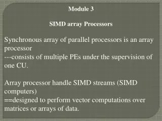
Introduction • Major characteristics of SIMD architectures • A single processor(CP) • Synchronous array processors(PEs) • Data-parallel architectures • Hardware intensive architectures • Interconnection network
Associative Processor • An SIMD whose main component is an associative memory.(Figure 2.19) • AM(Associative Memory): Figure 2.18 • Used in fast search operations • Data register • Mask register • Word selector • Result register
Introduction(continued) • Associative processor architectures also belong to the SIMD classification. • STRAN • Goodyear Aerospace’s MPP(massively parallel processor) • The systolic architectures are a special type of synchronous array processor architecture.
5.1 SIMD Organization • Figure 5.1 shows a SIMD processing model. (Compare to Figure 4.1) • Example 5.1 • SIMDs offer an N-fold throughput enhancement over SISD provided the application exhibits a data-parallelism of degree N.
5.1 SIMD Organization (continued) • Memory • Data are distributed among the memory blocks • A data alignment network allows any data memory to be accessed by any PE.
5.1 SIMD Organization (continued) • Control processor • To fetch instructions and decode them • To transfer instructions to PEs for executions • To perform all address computations • To retrieve some data elements from the memory • To broadcast them to all PEs as required.
5.1 SIMD Organization (continued) • Arithmetic/Logic processors • To perform the arithmetic and logical operations on the data • Each PE corresponding to data paths and arithmetic/logic units of an SISD processor capable of responding to control control signals from the control unit.
5.1 SIMD Organization (continued) • Interconnection network (Refer to Figure 2.9) • In type 1 and type 2 SIMD architectures, the PE to memory interconnection through n x n switch • In type 3, there is no PE-to-PE interconnection network. There is a n x n alignment switch between PEs and the memory block.
5.1 SIMD Organization (continued) • Registers, instruction set, performance considerations • The instruction set contains two types of index manipulation instructions, one set for global registers and the other for local registers
5.2 Data Storage Techniques and Memory Organization • Straight storage / skewed storage • GCD
5.3 Interconnection Networks • Terminology and performance measures • Nodes • Links • Messages • Paths: dedicated / shared • Switches • Directed(or indirect) message transfer • Centralized (or decentralized) indirect message transfer
5.3 Interconnection Networks (continued) • Terminology and performance measures • Performance measures • Connectivity • Bandwidth • Latency • Average distance • Hardware complexity • Cost • Place modularity • Regularity • Reliability and fault tolerance • Additional functionality
5.3 Interconnection Networks (continued) • Terminology and performance measures • Design choices(by Feng): refer to Figure 5.9 • Switching mode • Control strategy • Topology • Mode of operation
5.3 Interconnection Networks (continued) • Routing protocols • Circuit switching • Packet switching • Worm hole switching • Routing mechanism • Static / dynamic • Switching setting functions • Centralized / distributed
5.3 Interconnection Networks (continued) • Static topologies • Linear array and ring • Two dimensional mesh • Star • Binary tree • Complete interconnection • hypercube
5.3 Interconnection Networks (continued) • Dynamic topologies • Bus networks • Crossbar network • Switching networks • Perfect shuffle • Single stage • Multistage
5.4 Performance Evaluation and Scalability • The speedup S of a parallel computer system: • Theoretically, the maximum speed possible with a p processor system is p. ( A superlinear speedup is an exception) • Maximum speedup is not possible in practice, because all the processors in the system cannot be kept busy performing useful computations all the time.
5.4 Performance Evaluation and Scalability (continued) • The timing diagram of Figure 5.20 illustrates the operation of a typical SIMD system. • Efficiency, E is a measure of the fraction of the time that the processors are busy. In Figure 5.20, s is the fraction of the time spent in serial code. 0 E 1
5.4 Performance Evaluation and Scalability (continued) • The serial execution time in Figure 5.20 is one unit and if the code that can be run in parallel takes N time units on a single processor system, • The efficiency is also defines as
5.4 Performance Evaluation and Scalability (continued) • The cost is the product of the parallel run time and the number of processors. • Cost optimal: if the cost of a parallel system is proportional to the execution time of the fastest algorithm. • Scalability is a measure of its ability to increase speedup as the number of processors increases.
5.5 Programming SIMDs • The SIMD instruction set contains additional instruction for IN operations, manipulating local and global registers, setting activity bits based on data conditions. • Popular high-level languages such as FORTRAN, C, and LISP have been extended to allow data-parallel programming on SIMDs.
5.6 Example Systems • ILLIAC-IV • The ILLIAC-IV project was started in 1966 at the University of Illinois. • A system with 256 processors controlled by a CP was envisioned. • The set of processors was divided into four quadrants of 64 processors. • Figure 5.21 shows the system structure. • Figure 5.22 shows the configuration of a quadrant. • The PE array is arranged as an 8x8 torus.
5.6 Example Systems (continued) • CM-2 • The CM-2, introduced in 1987, is a massively parallel SIMD machine. • Table 5.1 summarizes its characteristics. • Figure 5.23 shows the architecture of CM-2.
5.6 Example Systems (continued) • CM-2 • Processors • The 16 processors are connected by a 4x4 mesh. (Figure 5.24) • Figure 5.25 shows a processing cell. • Hypercube • The processors are linked by a 12-dimensional hypercube router network. • The following parallel communication operations permit elements of parallel variables: reduce & broadcast, grid(NEWS), general(send, get), scan, spread, sort.
5.6 Example Systems (continued) • CM-2 • Nexus • A 4x4 crosspoint switch, • Router • It is used to transmit data from a processor to the other. • NEWS Grid • A two-dimensional mesh that allows nearest-neighbor communication.
5.6 Example Systems (continued) • CM-2 • Input/Output system • Each 8-K processor section is connected to one of the eight I/O channels (Figure 5,26). • Data is passed along the channels to I/O controller (Figure 5.27). • Software • Assembly language, Paris • *LISP, CM-LISP, and *C • Applications: refer to page 211.
5.6 Example Systems (continued) • MasPar MP • The MasPar MP-1 is a data parallel SIMD with basic configuration consisting of the data parallel unit(DDP) and a host workstation. • The DDP consists of from 1,024 to 16,384 processing elements. • The programming environment is UNIX-based. Programming languages are MDF(MasPar FORTRAN), MPL(MasPar Programming Language)
5.6 Example Systems (continued) • MasPar MP • Hardware architecture • The DPU consists of a PE array and an array control unit(ACU). • The PE array(Figure 5.28) is configurable from 1 to 16 identical processor boards. Each processor board has 64 PE clusters(PECs) of 16 PEs per cluster. Each processor board thus contains 1024 PEs.
5.7 Systolic Arrays • A systolic array is a special purpose planar array of simple processors that feature a regular, near-neighbor interconnection network.
Figure 5-31(iWarP System) • iWarp (Intel 1991) • Developed jointly by CMU and Intel Corp. • A programmable systolic array • Memory communication & systolic communication • The advantages of systolic communication • Fine grain communication • Reduced access to local memory • Increased instruction level parallelism • Reduced size of local memory
Figure 5-31(iWarP System) • An iWarp system is made of an array of iWarp cells • Each iWarp cell consists of an iWarp component and the local memory. • The iWarp component contains independent communication and computation agents