Demography
Demography. Introduction to Life Tables Logistic model approach provides a simple, general model, but important details missing. In a life table we incorporate the vital statistics of the species. In particular, age-specific birth and death rates.


Demography
E N D
Presentation Transcript
Introduction to Life Tables Logistic model approach provides a simple, general model, but important details missing. In a life table we incorporate the vital statistics of the species. In particular, age-specific birth and death rates. We will be able to analyze potential growth rates of a population. We will be able to estimate the life expectancy of an individual of known age.
Recall assumptions • r and K are constant • Environment will not change (physical and biotic) • Populations will not evolve • 2. All individuals are identical • Ages are equal • Sizes are equal • Genders are equal • 3. Populations are closed • No immigration • No emigration
Life Span Determinate versus indeterminate growth Fish and trees vs mice and butterflies; important when mortality correlated with size Importance of physical environment. Slow growth where temperature low or nutrients scarce
Survivorship of the lapwing Plotted on a semi-log plot. The straight line indicates a constant probability of death, regardless of age.
Life Tables x = age at beginning of the time interval Sx = Number of survivors at start of interval
Survivorship dx = Number dying during interval lx = Proportion surviving at start of age interval = nx/no
Age-specific survival and mortality rates gx = sx = px=age specific survival rate (probability of surviving to the end of the period) = nx+1/nx = lx+1/lx = (nx-dx)/nx mx = qx = age specific mortality rate (probability of dying before the end of the period) = (nx-(nx+1)) / nx = dx/nx = 1 - gx
Calculation of age-specific life expectancy Nx = Mean number of individuals alive during the period = (nx+nx+1)/2 Tx = sum of the time to be lived by the nx currently alive ex = age specific life expectancy
Exponential mortality rate kx = Exponential mortality = ln gx gx = e-kt
Types of mortality curves Three basic types of survivorship curves Semilog plot is Negative skewed = Type I Survivorship starts out high but then drops off quickly at older age Semilog plot is diagonal = Type IISurvivorship is constant with age Semilog plot is Positively skewed = Type III Survivorship very low for young individuals, but increases greatly with age Typically a blend with initial high drop, then diagonal, then senescence period.
Thar Introduced in New Zealand Type I
Roe deer in Denmark with marked differences in survivorship rates between genders
Mortality rates of grey seals. Observe the burden of being a mature male.
Density dependence in age-specific mortality rates of the African Buffalo.
Comparison of human survivorship in Rome and North Africa in the first four centuries A.D.
Comparisons of human life expectancy in various European populations
Survivorship in the sawfly, an insect species with a complex life history
Types of lifetable studies Age specific (horizontal or dynamic or cohort) life table; one cohort followed Time specific (vertical or static); one point in time – a snapshot view Composite age specific; remains of dead Three not equivalent unless stable population.
Gross Reproductive Rate Fecundity at age x = bx Gross reproductive rate (GRR) = Σ bx
Net Reproductive Rate lxbx = Number of female individuals born during interval x. Net Reproductive Rate (average number)=Ro=lxbx=( Fx)/no
Projection of Population Size Population at time t and age x = Nt(x) Where x>1, Nt(x) = (N(t-1)(x-1))(sx-1) Where x=1, Nt(1) = i=1,∞ (N(t-1)(i))(bi)
G = cohort generation length = mean period elapsing between birth of parent and birth of offspring. G = [(lxbxx)]/[(lxbx)] = 2.1/1.2 = 1.75 = (xFx)/Fx (The time it takes) / (number produced)
Calculation of r • Recall Nt = Noert; • set t=G NG/No = erG ~ Ro • ln(NG/No) = lnRo ~ rG • r ~ ln(Ro)/G = ln(1.2)/1.75 = .104 • recall G = (xlxbx)/ (lxbx) =(xlxbx)/ Ro • r ~ (RolnRo)/ (xlxbx)
Reproductive value vx = [erx/lx][ (e-rxlyby)] ; where summation over range y = x → ∞
Applications? Population projections? Sensitivity analysis? Conservation strategies?
Elephant seals: McMahon et al. 2005 The dynamics of animal populations are determined by several key demographic parameters, which vary over time with resultant changes in the status of the population. When managing declining populations, the identification of the parameters that drive such change are a high priority, but are rarely achieved for large and long-lived species. Southern elephant seal populations in the South Indian and South Pacific oceans have decreased by as much as 50% during the past 50 yr. The reasons for these decreases remained unknown. This study used a projected stochastic Leslie-matrix model based on long-term demographic data to examine the potential role of several life-history parameters in contributing to the declines. The models simulated the observed population trends that were independently derived from annual abundance surveys.