Chapter 8 Interconnection Networks and Clusters

1. EEF011 Computer Architecture計算機結構 Chapter 8Interconnection Networks and Clusters 吳俊興 高雄大學資訊工程學系 January 2005

2. Chapter 8. Interconnection Networks and Clusters 8.1 Introduction 8.2 A Simple Network 8.3 Interconnection Network Media 8.4 Connecting More Than Two Computers 8.5 Network Topology 8.6 Practical Issues for Commercial Interconnection Networks 8.7 Examples of Interconnection Networks 8.8 Internetworking 8.9 Crosscutting Issues for Interconnection Networks 8.10 Clusters 8.11 Designing a Cluster 8.12 Putting it All Together: The Google Cluster of PCs

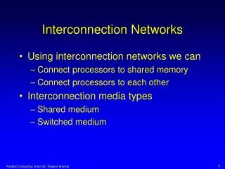
3. 8.1 Introduction • Networks • Goal: Communication between computers • Eventual Goal: treat collection of computers as if one big computer, distributed resource sharing • Why devote attention to networking for architects • Use a network to connect autonomous systems within a computer • switches are replacing buses • Almost all computers are, or will be, networked to other devices • Warning: terminology-rich environment

4. Networks Facets people talk a lot about: • direct (point-to-point) vs. indirect (multi-hop) • networking vs. internetworking • topology (e.g., bus, ring, DAG) • routing algorithms • switching (aka multiplexing) • wiring (e.g., choice of media, copper, coax, fiber)

5. Interconnection Networks • Examples • Wide Area Network (ATM): 100-1000s nodes; ~ 5,000 km • Local Area Networks (Ethernet): 10-1000 nodes; ~ 1-2 km • System/Storage Area Networks (FC-AL): 10-100s nodes; ~ 0.025 to 0.1 km per link cluster: connecting computers RAID: connecting disks SMP: connecting processors

6. 8.2 A Simple Network • Starting Point: Send bits between 2 computers • Queue (FIFO) on each end • Information sent called a “message” • Can send both ways (“Full Duplex”) • Rules for communication? “protocol” • Inside a computer: • Loads/Stores: Request (Address) & Response (Data) • Need Request & Response signaling

7. A Simple Example • What is the format of message? • Fixed? Number bytes? 0: Please send data from Address 1: Packet contains data corresponding to request Header/Trailer: information to deliver a message Payload: data in message (1 word above)

8. Questions About Simple Example • What if more than 2 computers want to communicate? • Need computer “address field”(destination) in packet • What if packet is garbled in transit? • Add “error detection field”in packet (e.g., Cyclic Redundancy Check) • What if packet is lost? • More “elaborate protocols”to detect loss (e.g., NAK, ARQ, time outs) • What if multiple processes/machine? • Queue per process to provide protection • Simple questions such as these lead to more complex protocols and packet formats => complexity

9. A Simple Example Revised • What is the format of packet? • Fixed? Number bytes? • Send a message: • The application copies data to be sent into an OS buffer • The OS calculates the checksum, includes it in the head or trailer of the message, and then starts the timer • The OS sends the data to the network interface hardware and tells the hardware to send the message • Receive a message: • The system copies the data from the network interface hardware into OS buffer • The OS calculates the checksum over the data. If the checksum matches the senders checksum, sends an ACK back to the sender. If not, deletes the message • If the data pass the test, the OS copies the data to the user’s address space

10. Network Performance Measures Overhead: latency of interface vs. Latency: network

11. Sender Overhead Transmission time (size ÷ bandwidth) Universal Performance Metrics Sender (processor busy) Time of Flight Transmission time (size ÷ bandwidth) Receiver Overhead Receiver (processor busy) Transport Latency Total Latency Total Latency = Sender Overhead + Time of Flight+ Message Size ÷ BW +Receiver Overhead Includes header/trailer in BW calculation?

12. Figure 8.8 Bandwidth delivered vs. message sizefor 25 and 250 us overheads and for 100, 1000, and 10,000M bits/sec bandwidths Bandwidth delivered vs. message size for overheads of 25 and 250 us and for network bandwidths of 100, 1000, and 10,000M bits/sec message size must be greater than 256 bytes for the effect bandwidth to exceed 10M bits/sec

13. Figure 8.9 Cumulative % of messages and data transferred as message size varies for NFS traffic Each x-axis entry includes all bytes up to the next one; eg., 32 means 32 to 63 bytes More than half the bytes are sent in 8 KB messages, but 95% of the messages are less than 192 bytes

14. Figure 8.10 Cumulative % of messages and data transferred as message size varies for Internet traffic About 40% of the messages were 40 bytes long, and 50% of the data transfer was in messages 1500 bytes long. The MAX transfer unit of most switches was 1500 bytes

15. 8.3 Interconnect Network Media Network Media Copper, 1mm think, twisted to avoid attenna effect (telephone). "Cat 5" is 4 twisted pairs in bundle Used by cable companies: high BW, good noise immunity Light: 3 parts: cable, light source, light detector. Note fiber is unidirectional; need 2 for full duplex

16. Fiber Optics • Multimode fiber: ~ 62.5 microns in diameter • vs. the 1.3 micron wavelength of infrared light • Use inexpensive LEDs as a light source: LEDs and dispersion limit its length at 1000 Mbits/s for 0.1 km, and 1-3 km at 100 Mbits/s • wider  more dispersion problems: some wave frequencies have different propagation velocities • Single mode fiber: "single wavelength" fiber (8-9 microns) • Use laser diodes, 1-5 Gbits/s for 100s kms • Less reliable and more expensive, and restrictions on bending • Cost, bandwidth, and distance of single-mode fiber affected by • power of the light source • the sensitivity of the light detector, and • the attenuation rate (loss of optical signal strength as light passes through the fiber) per kilometer of the fiber cable • Typically glass fiber, since has better characteristics than the less expensive plastic fiber

17. Wave Division Multiplexing Fiber • Wave Division Multiplexing (WDM): • Send N independent streams • on the same single fiber using different wavelengths of light, and then • demultiplexes the different wavelengths at the receiver • WDM in 2001: 40 Gbit/s using 8 wavelengths • Plan to go to 80 wavelengths => 400 Gbit/s! • A figure of merit: BW* max distance (Gbit-km/sec) • 10X/4 years, or 1.8X per year

18. Compare Media • Assume 40 2.5" disks, each 25 GB, Move 1 km • Compare Cat 5 (100 Mbit/s), Multimode fiber (1000 Mbit/s), single mode (2500 Mbit/s), and car • Cat 5: 1000 x 1024 x 8 Mb / 100 Mb/s = 23 hrs • MM: 1000 x 1024 x 8 Mb / 1000 Mb/s = 2.3 hrs • SM: 1000 x 1024 x 8 Mb / 2500 Mb/s = 0.9 hrs • Car: 5 min + 1 km / 50 kph + 10 min = 0.25 hrs • Car of disks = high BW media

19. 8.4 Connecting More Than Two Computers Shared media: share a single interconnection • just as I/O devices share a single bus • broadcast in nature: easier for broadcast/multicast • Arbitration in Shared network? • Central arbiter for LAN: not scalable • Carrier Sensing: listen to check if being used • Collision Detection: listen to check if collision • Random Back-off: resend to avoid repeated collisions; not fair arbitration Switched: media: point-to-point connections • point-to-point is faster since no arbitration, simpler interface • pairs communicate at same time • Aggregate BW in switched network is many times that of a single shared medium • also known as data switching interchanges, multistage interconnection networks, interface message processors

20. Connection-oriented vs. Connectionless • Connection-oriented: establish a connection before communication • Telephone: operator sets up connection between a caller and a receiver • Once connection established, conversation can continue for hours, even silent • Share transmission lines over long distances by using switches to multiplex several conversations on the same lines • Frequency division multiplexing: divide B/W transmission line into a fixed number of frequencies, with each frequency assigned to a conversation • Time division multiplexing: divide B/W transmission line into a fixed number of slots, with each slot assigned to a conversation • Problem: lines busy based on # of conversations, not amount of information sent • Advantage: reserved bandwidth (QoS) • Connectionless: every package of information has an address • Each package (packet) is routed to its destination by looking at its address • Analogy, the postal system (sending a letter) • also called “Statistical multiplexing” • Circuit switching vs. Packet switching

21. Routing: Delivering Messages • Shared Media: broadcast to everyone • Each node checks whether the message is for that node • Switched Media: needs real routing. Three options: • Source-based routing: message specifies path to the destination (changes of direction) • Virtual Circuit: circuit established from source to destination, message picks the circuit to follow, ex. ATM • Destination-based routing: message specifies destination, switch must pick the path • deterministic: always follow the same path • adaptive: the network may pick different paths to avoid congestion or failures • Randomized routing: pick between several good paths to balance network load • spread the traffic throughout the network, avoiding hot spots

22. 110 010 111 011 100 000 101 001 Deterministic Routing Examples • mesh: dimension-order routing • (x1, y1) → (x2, y2) • first x = x2 -x1, • then y = y2 -y1, • hypercube: edge-cube routing • X = xox1x2 . . .xn → Y = yoy1y2 . . .yn • R = X xor Y • Traverse dimensions of differing address in order • tree: common ancestor

23. Store-and-Forward vs. Worm-hole Routing • Store-and-forward policy: each switch waits for the full packet to arrive in switch before sending to the next switch (good for WAN) • Cut-through routing or worm hole routing: switch examines the header, decides where to send the message, and then starts forwarding it immediately • In worm hole routing, when head of message is blocked, message stays strung out over the network, potentially blocking other messages (needs only buffer the piece of the packet that is sent between switches). • Cut through routing lets the tail continue when head is blocked, compressing the whole strung-out message into a single switch. (Requires a buffer large enough to hold the largest packet) • Advantage: Latency reduces from function of:number of intermediate switches * y the size of the packet totime for 1st part of the packet to negotiate the switches + the packet size ÷ interconnect BW

24. Congestion Control • Packet switched networks do not reserve bandwidth; this leads to contention(connection based limits input) • Solution: prevent packets from entering until contention is reduced (e.g., freeway on-ramp metering lights) • Three schemes for congestion control: • Packet discarding: If packet arrives at switch and no room in buffer, packet is discarded (e.g., UDP) • Flow control: between pairs of receivers and senders; use feedback to tell sender when allowed to send next packet • Back-pressure: separate wires to tell to stop • Window: give original sender right to send N packets before getting permission to send more; overlaps latency of interconnection with overhead to send & receive packet (e.g., TCP), adjustable window • Choke packets: aka “rate-based”; Each packet received by busy switch in warning state sent back to the source via choke packet. Source reduces traffic to that destination by a fixed % (e.g., ATM)

25. 8.5 Network Topology • Huge number of topologies developed • Topology matters less today than it did in the past • Common topologies • Centralized switch: separate from the processor and memory • fully connected: crossbar and omega • tree: fat tree multistage switch: multiple steps that a message may travel • Distributed switch: small switch at every processor • ring • grid or mesh • torus • hypercube tree

26. Centralized Switch - Crossbar • fully connected interconnection • any node to communicate with any other node in one pass through the interconnection • routing: depend on addressing • source-based: specified in the message • destination-based: a table decides which port to take a given address • uses n2 switches, where n is the number of processors • n = 8  8*8=64 switches • can simultaneously route any permutation of traffic pattern between processors unidirectional links

27. Centralized Switch – Omega Network • fully connected interconnection • less hardware: uses n/2 log2n switch boxes, each composed of 4 of the smaller switches • n = 8  4* (8/2 log28) = 4 * (4*3) = 48 switches • contention is more likely • e.g., P1 to P7 blocks while waiting for a message from P0 to P6 • cannot simultaneously route between any pairs of processors

28. Centralized Switch – Fat Tree • bandwidth added higher in the tree • redundancy help with fault tolerance and load balance • multiple paths between any two nodes in a fat tree • e.g. 4 paths between node 0 and node 8 • randomly routing would spread the load and result in fewer congestion • shaded circles are switches and squares are processors • simple 4-ary tree • e.g. CM-5

29. Distributed Switch - Ring • Full interconnection • n switches for n nodes • relay: some nodes are not directly connected • capable of many simultaneous transfers: node 1 can send to node 2 at the same time node 3 can send to node 4 • Long latency • Average message must travel through n/2 switches • Token ring: a single token for arbitration to determine which node is allowed to send a message

30. Distributed Switches – Mesh, Torus, Hypercube • bisection bandwidth: • divide the interconnect into two roughly equal parts, each with half the nodes • sum the bandwidth of the lines that cross the imaginary dividing line

31. 8.6 Practical Issues for Commercial Interconnection Networks • Connectivity • max number of machines affects complexity of network and protocols since protocols must target largest size • Interface - Connecting the network to the computer • Where in bus hierarchy? Memory bus? Fast I/O bus? Slow I/O bus? • (Ethernet to Fast I/O bus, Infiniband to Memory bus since it is the Fast I/O bus) • SW Interface: does software need to flush caches for consistency of sends or receives? • Programmed I/O vs. DMA? Is NIC in uncachable address space? • Standardization: cross-company interoperability • Standardization advantages: • low cost (components used repeatedly) • stability (many suppliers to chose from) • Standardization disadvantages: • Time for committees to agree • When to standardize? • Before anything built? => Committee does design? • Too early suppresses innovation • Message failure tolerance • Node failure tolerance

32. 8.7 Examples of Interconnection Networks All three have destination and checksum cell = message T: type field

33. Ethernets and Bridges • 10M bps standard proposed in 1978 and 100M bps in 1994 • Bridges, routers or gateways, hubs

34. Examples

35. 8.10 Clusters • Opportunities • LAN-switches: high network bandwidth, scalable, off the shelf component • 2001 Cluster = collection of independent computers using switched network to provide a common service • "loosely coupled“ applications (vs. shared memory applications) • databases, file servers, Web servers, simulations, and batch processing • Often need to be highly available, requiring error tolerance and repairability • Often need to scale • Challenges and drawbacks • Administration cost • administering a cluster of N machines ~ administering N independent machines • administering a SMP of N processor ~ administering 1 big machine • Communication overhead • Clusters connected using I/O bus: expensive communication, conflict with other I/O traffic • SMP connected on memory bus: higher bandwidth, much lower latency • Division of memory • Cluster of N machines has N independent memories and N copies of OS • SMP allows 1 program to use almost all memory • DRAM prices has made memory costs so low that this multiprocessor advantage is much less important in 2001

36. Cluster Advantages Dependability and Scalability Advantages • Error isolation: separate address space limits contamination of error • Repair: Easier to replace a machine without bringing down the system than in an shared memory multiprocessor • Scale: easier to expand the system without bringing down the application that runs on top of the cluster • Cost: Large scale machine has low volume => fewer machines to spread development costs vs. leverage high volume off-the-shelf switches and computers • Amazon, AOL, Google, Hotmail, Inktomi, WebTV, and Yahoo rely on clusters of PCs to provide services used by millions of people every day

37. Popularity of Clusters Figure 8.30 Plot of top 500 supercomputer sites between 1993 and 2000(> 100 tera-FLOPS in 2001) • Clusters grew from 2% to almost 30% in the last three years, while uniprocessors and SMPs have almost disappeared • Most of the MPPS look similar to clusters

38. 8.11 Designing a Cluster • Designing a system with about 32 processors, 32 GB of DRAM, and 32 or 64 disks using Figure 8.33 • Higher price for processors and DRAM • Base configuration: 256MB DRAM,2 100Mb Ethernets, 2 disks, a CD-ROM drive, a floppy drive, 6-8 fans, and SVGA graphics

39. Four Examples • Cost of cluster hardware alternatives with local disk • The disks are directly attached to the computers in the cluster • 3 alternatives: building from a uniprocessor, a 2-way SMP, and an 8-way SMP • Cost of cluster hardware alternatives with disks over SAN • Move the disk storage behind a RAID controller on a SAN • Cost of cluster options that is more realistic • Includes costs of software, space, maintenance, and operator • Cost and performance of a cluster for transaction processing • Examine a database-oriented cluster using TPC-C benchmark

40. Example 1. Cluster with Local Disk Figure 8.34 three cluster organizations Overall cost: 2-way < 1 way < 8-way • Expansibility incurs high prices • 1 CPU+ 512MB DRAM in 8-way SMP costs more than that in 1-way • Network vs. local bus trade-off • 8-way spends less on networking

41. Example 2. Using a SAN for Disks • Problem with Example 1 • no protection against a single disk failure • local state managed separately The system is down on a disk failure • Centralize the disks behind a RAID controller using FC-AL as the SAN (FC-AL SAN + FC-AL disks) • RAID 5: 28+8 disks • Costs of both LAN network and SAN decrease as the # of computers in the cluster decreases Figure 8.36 Components for storage area network

42. Example 3. Accounting for Other Costs Additional costs for the operation • software cost • cost of a maintenance agreement for hardware • cost of the operators • In 2001, $100,000 per year for an operator • Operator costs are as significant as purchase price Fig. 8.39 Total cost of ownership for 3 years for clusters in Example 1 and Example 2

43. Example 4.A Cluster for Transaction Processing • IBM cluster for TPC-C. 32 P-III@900 MHz processors, 32*4GB RAM. • Disks: 15,000 RPM • 8 TB / 728 disks: 560@9.1GB + 160@18.2GB + 8@9.1GB (system) • 14 disks/enclosure * 13 enclosures /computer * 4

44. Figure 8.41 Comparing 8-way SAN cluster andTPC-C cluster in price (in $1000s) and percentage • Higher cost of CPUs • More total memory • higher capacity • Higher cost of software: SQL server + IBM software installation • Higher maintenance cost: IBM setup cost

45. 8.12 Putting it all together: Google • Google: search engines: 24x7 availability • 12/2000: 70M queries per day, or AVERAGE of 800 queries/sec all day • Response time goal: < 1/2 sec for search • Google crawls WWW and puts up new index every 4 weeks • Stores local copy of text of pages of WWW (snippet, cached copy of page) • 3 collocation sites (2 CA + 1 Virginia) • 6000 PCs, 12000 disks: almost 1 petabyte! • 2 IDE drives, 256 MB of SDRAM, modest Intel microprocessor, a PC mother-board, 1 power supply and a few fans • Each PC runs the Linix operating system • Buy over time, so upgrade components:populated between March and November 2000 • microprocessors: 533 MHz Celeron to an 800 MHz Pentium III, • disks: capacity between 40 and 80 GB, speed 5400 to 7200 RPM • bus speed is either 100 or 133 MH • Cost: ~ $1300 to $1700 per PC • PC operates at about 55 Watts • Rack => 4500 Watts , 60 amps

46. Hardware Infrastructure • VME rack 19 in. wide, 6 feet tall, 30 inches deep • Per side: 40 1 Rack Unit (RU) PCs +1 HP Ethernet switch (4 RU): Each blade can contain 8 100-Mbit/s EN or a single 1-Gbit Ethernet interface • Front+back => 80 PCs + 2 EN switches/rack • Each rack connects to 2 128 1-Gbit/s EN switches • Dec 2000: 40 racks at most recent site

47. Reliability • For 6000 PCs, 12000s, 200 EN switches • ~ 20 PCs will need to be rebooted/day • ~ 2 PCs/day hardware failure, or 2%-3% / year • 5% due to problems with motherboard, power supply, and connectors • 30% DRAM: bits change + errors in transmission (100 MHz) • 30% Disks fail • 30% Disks go very slow (10%-3% expected BW) • 200 EN switches, 2-3 fail in 2 years • 6 Foundry switches: none failed, but 2-3 of 96 blades of switches have failed (16 blades/switch) • Collocation site reliability: • 1 power failure,1 network outage per year per site • Bathtub for occupancy

48. Google Performances Serving • How big is a page returned by Google? ~16KB • Average bandwidth to serve searches 70,000,000/day x 16,750 B x 8 bits/B 24 x 60 x 60 =9,378,880 Mbits/86,400 secs = 108 Mbit/s Crawling • How big is a text of a WWW page? ~4000B • 1 Billion pages searched; Assume 7 days to crawl • Average bandwidth to crawl 1,000,000,000/pages x 4000 B x 8 bits/B 24 x 60 x 60 x 7 =32,000,000 Mbits/604,800 secs = 59 Mbit/s Replicating Index • How big is Google index? ~5 TB • Assume 7 days to replicate to 2 sites, implies BW to send + BW to receive • Average bandwidth to replicate new index 2 x 2 x 5,000,000 MB x 8 bits/B 24 x 60 x 60 x 7 =160,000,000 Mbits/604,800 secs = 260 Mbit/s

49. Summary Chapter 8. Interconnection Networks and Clusters 8.1 Introduction 8.2 A Simple Network 8.3 Interconnection Network Media 8.4 Connecting More Than Two Computers 8.5 Network Topology 8.6 Practical Issues for Commercial Interconnection Networks 8.7 Examples of Interconnection Networks 8.8 Internetworking 8.9 Crosscutting Issues for Interconnection Networks 8.10 Clusters 8.11 Designing a Cluster 8.12 Putting it All Together: The Google Cluster of PCs