Download
1 / 31
310 likes | 576 Views
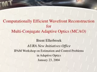
Computationally Efficient Wavefront Reconstruction for Multi-Conjugate Adaptive Optics (MCAO). Brent Ellerbroek AURA New Initiatives Office IPAM Workshop on Estimation and Control Problems in Adaptive Optics January 23, 2004. Presentation Outline. Anisoplanatism and MCAO

E N D
Computationally Efficient Wavefront ReconstructionforMulti-Conjugate Adaptive Optics (MCAO) Brent Ellerbroek AURA New Initiatives Office IPAM Workshop on Estimation and Control Problems in Adaptive Optics January 23, 2004
Presentation Outline • Anisoplanatism and MCAO • Minimum variance wavefront reconstruction methods for MCAO • Formulation, analytical solution, and scaling issues • Computationally efficient methods for very high-order MCAO systems • Spatial frequency domain modeling (Tokovinin) • Sparse matrix techniques • Conjugate gradients with multigrid preconditioning • Sample simulation results • MCAO Performance scaling with telescope diameter • Summary, acknowledgements, references
Anisoplanatism and Adaptive Optics • Bright guidestars are needed for wavefront sensing • Not enough bright natural stars for astronomical applications • Progress is being made in using lasers to generate artificial stars • Even with lasers, the corrected field-of-view is limited • Turbulence is 3-dimensional • One deformable mirror provides correction in a single direction • Anisoplanatism
Adaptive Optics Imagery with Anisoplanatism 23” • Low-order AO system on the Gemini-North telescope • Ambient seeing: 0.9” • AO-compensated seeing: 0.12” (center of field) to 0.19” (corner) • Impact increases as the quality of correction improves
MCAO Compensates Turbulence in Three Dimensions Wave Front Sensors (WFSs) Deformable Mirrors (DMs) Telescope Guide Stars (NGS or LGS) Atmospheric Turbulence • An application of limited angle tomography Processors and Control Algorithms
Sample MCAO Simulation Result MCAO Classical AO Strehl Guide star offset, arc sec • 8 meter telescope • 2 deformable mirrors with 13 by 13 actuators • 5 wavefront sensors with 12 by 12 subapertures
Wavefront Reconstruction for MCAO is Challenging • Multiple turbulence layers, deformable mirrors, wavefront sensors • Richer cross-coupling between variables • Higher dimensionality estimation problem • Especially for future extremely large telescopes! • Wide-field performance evaluation and optimization
Wavefront Reconstruction as a Linear Inverse Problem • Quantities of interest • Turbulence profile x… • …to be corrected by a DM actuator command vector a… • … using a WFS measurement s with noise component n… • …leaving a residual phase error f with mean-square value s2 • Relationships • s = Gx + n (wavefront sensing) • a = Rs (wavefront reconstruction) • f = Hxx – Haa (residual error computation) • s2 = fTWf (variance evaluation) • Objective: Select R to (in some sense) minimize s2
Minimum Variance Wavefront Reconstruction • Model x, s, and n as zero mean random variables with finite second moments • Select R to minimize (the expected value of s2): • Partials of with respect to Rij must vanish at R=R* • Solution given by R*=F*E*, where
Interpretation (and Use) of R* = F*E* • Interpretation • E* is the “turbulence Estimation matrix” • Minimum variance estimate of profile x from measurement s • Depends upon WFS geometry, statistics of x and s • Independent of the DM geometry • F* is the “turbulence Fitting matrix” • RMS best fit to estimated value of x using DM degrees of freedom • Independent of WFS geometry, statistics of x and s • Depends upon the DM geometry • Use • Once R* is known, we can estimate performance using • …or we can use R* to run simulations (or even systems)
Computational Complexity • R* has complexity O(N3) to explicitly compute and evaluate, complexity O(N2) to apply in real time • Must be computed/evaluated in a few hours for studies • Must be applied at rates of 1-2 KHz for actual use • Current generation MCAO systems have N < 1000 • Computationally feasible • Proposed MCAO systems have N > 104 or 105 • Explicit computations inefficient or outright infeasible • How do we analyze and simulate such systems???
Analytical Methods in the Spatial Frequency Domain • Wavefront propagation, sensing, correction, and reconstruction are all approximately spatial filtering operations • Filtering representation becomes exact in the limit of an infinite aperture AO system • Wavefront reconstruction decouples into small independent problems at each spatial frequency • Each problem has dimensionality 2 Nwfs by Ndm • Overall complexity scales as O(Nfreq) aO(N) • Analytical method only, but very useful
Efficient Approaches for the Spatial Domain • Must solve Ax=y, where without explicitly computing A-1 • Exploit matrix structure • G, Ha, W are sparse • is diagonal (plus a low-rank perturbation due to laser guide star position uncertainty) • has good approximations that are sparse • Efficient solutions possible • Sparse matrix techniques (close, but not quite) • Conjugate gradients with multigrid preconditioning
G, H Sparse for Nodal Representations of Turbulence • Each value of f (r) is determined by turbulence values along a single ray path • Each WFS measurement si is determined by values of f(r) within a small subaperure Si f(r)
Sparse Matrix Methods • Suppose A is sparse (with bandwidth O(N1/2)) • Factor A = LLT where L is sparse and lower triangular • Solve Ax=y in two steps: Lx’ = y, followed by LTx = x’ • Complexity reduced from O(N2) to O(N3/2) • Complexity further reduced by reording rows/columns of A • For F*, is sparse (at least for conventional AO) • For E*, isn’t sparse for two reasons: • The turbulence covariance matrix isn’t sparse • For laser guidestars, is the sum of sparse and low rank terms
Sparse Approximation to Turbulence Statistics • is block diagonal, with Nlayer by Nlayer blocks • Each diagonal block is full rank! • We approximate block j as • ai proportional to layer strength • D is a discrete (and sparse) approximation to • Heuristic justification #1: • Both and DTD suppress high spatial frequencies • Heuristic justification #2: • In the spatial frequency domain
LGS Measurement Noise • For a LGS WFS, n is determined by two effects: • Detector readout noise and photon statistics (uncorrelated) • LGS position uncertainty on the sky • Two dimensions of uncertainty per guidestar, correlated between subapertures • More formally • UUT is a non-sparse matrix of rank 2 NLGS • Sparse matrix methods are not immediately applicable
Applying the Matrix Inversion Lemma • is the sum of and a low rank term UUT • Can solve by solving and adding a perturbation term depending upon Sparse Low Rank
Sample Matrix Factorizations for E* A matrix Cholesky Factor 0.03% Fill 1.65% Fill Cholesky Factor Reordered A 0.33% Fill 0.03% Fill • Conventional AO with 1 DM and 1 WFS!
MCAO Increases Coupling between Turbulence Layers • However, the coupling within a single layer is no greater than before f(r’,q’) f(r,q)
G, H Matrices Are Block Structured for MCAO • Column block structure due to multiple atmospheric layers • Row block structure due to multiple stars/guidestars G (5 guidestars, 6 atmospheric layers) Ha (3 mirrors, 25 stars)
Cross-Coupling of Atmospheric Layers for MCAO • Fill-in of “sparse” Cholesky factorization exceeds 10% • Cannot factor matrices for a 32m diameter system in a 2 Gbyte address space
An “Efficient” MCAO Reconstruction Algorithm • Biggest challenge is solving Ax=y with • Minimize ||Ax-y||2 using conjugate gradients • Use multigrid preconditioning to accelerate convergence • Preconditioning: Solve an approximate system A’x=y once per conjugate gradient cycle • Multigrid: Solution to A’x=y determined on multiple spatial scales to accelerate convergence at all spatial frequencies • Solution on each multigrid scale is determined using a customized (new?) technique: • Block symmetric Gauss-Seidel iterations on Ax=y • Block structure derived from atmospheric layers • Sparse matrix factorization of diagonal blocks
Block Symmetric Gauss-Seidel Iterations • Blocks of A, x, y denoted as Aij, xi, yj • Decompose A = L + D + U into a sum of lower triangular, diagonal, and upper triangular blocks • Iterative solution to Ax = (L+D+U)x = y given by (L+D)x’(n) = y – Ux(n) (U+D)x(n+1) = y – Lx’(n) • Solve for x’(n) and x(n+1) one block at a time: • Solve systems Diu=v using sparse Cholesky factorizations
MCAO Simulations for Future Telescopes • Goal: Evaluate MCAO performance scaling with aperture diameterD from D=8m to D=32m • Consider Natural, Sodium, and Rayleigh guidestars • Other simulation parameters: • Cerro Pachon turbulence profile with 6 layers • 1 arc minute square field-of-view • 3 DM’s conjugate to 0, 5.15, and 10.30 km • Actuator pitches of 0.5, 0.5, and 1.0 m • 5 higher order guidestars at corners and center of 1’ field • 0.5 m subapertures • 4 tip/tilt NGS WFS for laser guide star cases • 10 simulation trials per case using 64 m turbulence screens with 1/32m pitch
Sample Numerical Results Rayleigh Laser guidestars, h=30 km Sodium laser guidestars, h=90 km Natural guidestars
CG Convergence Histories • Rapid convergence for first 20 iterations • Convergence then slows due to poor conditioning of A • Not an issue for practical simulations • Results effectively independent of aperture diameter and guide star type
Summary • MCAO compensates anisoplanatism and corrects for the effects of atmospheric turbulence across extended fields-of-view • Minimum variance estimation is a viable approach to MCAO wavefront reconstruction • Computationally efficient methods needed for the very high order systems proposed for future extremely large telescopes • Conjugate gradient wavefront reconstruction using multigrid preconditioning and block symmetric Gauss-Seidel iterations enables simulations of 32 meter MCAO systems with 30k sensor measurements and 8k mirror actuators • Challenging problems remain • Closed-loop wavefront reconstruction and control • Hardware and software for real-time implementation
Acknowledgements • Luc Gilles and Curt Vogel • Ongoing collaboration on efficient methods • Matrix sparsity plots • Francois Rigaut • MCAO figure and performance plot • Gemini Observatory • Sample AO results • Support from AFOSR, NSF, and CfAO
References • Adaptive optics websites • CfAO, http://cfao.ucolick.org • Gemini AO web pages at http://www.gemini.edu • Minimum variance wavefront reconstruction • Wallner, JOSA 73, 1771 (1983) • Ellerbroek, JOSA A 11, 783 (1994) • Fusco et al., JOSA A 18, 2527 (2001) • Efficient implementations • Ellerbroek, JOSA A 19, 1803 (2002) • Ellerbroek, Gilles, Vogel, SPIE Proc. 4839, 989 (2002) • Gilles, Ellerbroek, Vogel, Appl. Opt. 42, 5233 (2003)