Download
1 / 50
500 likes | 771 Views
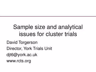
Sample size and analytical issues for cluster trials. David Torgerson Director, York Trials Unit djt6@york.ac.uk www.rcts.org. Background.

E N D
Sample size and analytical issues for cluster trials David Torgerson Director, York Trials Unit djt6@york.ac.uk www.rcts.org
Background • For any trial we want to make it sufficiently large that if there were a ‘true’ difference between the groups that this difference would be statistically significant. • A Type II error occurs when we wrongly conclude there is no difference when there actually is.
Sample size calculations • “Most hand calculations diabolically strain human limits, even for the easiest formula,..” (Schulz & Grimes, Lancet 2005)
Sample size formulae • Usually need a computer to calculate. However, a simple approximation for a two armed randomised trial with 1:1 ratio for a continuous variable (e.g., blood pressure) is as follows d = effect size (difference/standard deviation):
Example • We want to investigate a treatment for back pain. The measure is the Roland and Morris back pain scale with a standard deviation of 4. If we want to detect a 2 point difference how many do we need? • 2/4 = 0.5 = Effect size (d). 0.5 x 0.5 = 0.25. • 32/0.25 = 128 in total for 80% power, 5% significance (use 42 for 90% power). • NB using computer software answer = 126
Binary variables • For a dichotomous variable (cured not cured) the following is useful (a = average proportion difference).
Example • Breast feeding rates are only 50% and we have an educational intervention where we think this will increase to 60%; how many do we need? • d2 = 0.6-0.5 = 0.12 = 0.01 • a = 0.6+0.5/2 = 0.55 • a2 = 0.552 = 0.3025 • 0.01/(0.55-0.3025) = 0.040 • 32/0.040 = 792 • Need 792 to have 80% power to show a 10% difference in breast feeding rates if it were present (use 42 for 90% power). • NB using computer software the answer is: 774
Approximations • The formulae slightly overestimate the true sample size needed. But they can be done on a hand calculator and you can impress the statisticians. • What about cluster trials?
Cluster Sample Size • Usual sample size estimates assume independence of observations. When people are members of the same cluster (e.g., classroom, GP surgery) they are more related than we would expect to be at random. • This is the intra-cluster correlation co-efficient.
ICC • The ICC needs to incorporated into the sample size calculations. The formula is as follows: Design effect = 1 + (m – 1) X ICC. Design effect is the size the sample needs to be inflated by. M is the number of people in the cluster.
Sample size example. • Let’s assume for an individually randomised trial we need 128 people to detect 0.5 of an effect size with 80% power (2p = 0.05). Now assume we have 24 groups with 7 members. The ICC is 0.05, which is quite high. • 1+ (7 – 1) x 0.05 = 1.3, we need to increase the sample size by 30%. Therefore, we will need 166 participants.
What happens if cluster gets bigger? • If our cluster size is twice as big (14), things begin to get really interesting. • 1+(14-1)x0.05 = 1.65. • What about 30? (1+(30-1)x 0.05 = 2.45 (I.e, 314 participants). • Say we randomise a larger cluster, such as a school (n = 500) (1+(500-1) x 0.05 = 25.95 (ie. 3322).
ICC size • ICCs can be large for some things. ICCs for educational outcomes for examples are often around 0.4 to 0.5. • A class-based RCT with n = 30 and an ICC of 0.4 would need 1,612 participants or 54 classes with n = 30 in each class.
What makes the ICC large? • If the treatment is applied to health care provider (e.g., guidelines will increase ICCs for patients). • If cluster relates to outcome variable (e.g., smoking cessation and schools) • If members of cluster are expected to influence each other (e.g., households).
Sample Size Problems Cluster Trials Demand Larger Sample Sizes
Conditional ICC • The key ICC is the conditional ICC, usually we only have access to estimates of the unconditional ICC. • If we know, and can measure, characteristics that cause the ICC, we can adjust for this and lower the ICC. • Cook claims that using covariates allows a school based RCT to reduce the number for schools from about 50 to around 22.
Summary of sample size • The KEY thing is the size of the cluster. It is nearly always best to get lots of small clusters than a few large ones (e.g, a trial with small hospital wards, GP practices, classrooms will, ceteris paribus, be better than large clusters). • BUT if the ICC is tiny may not affect the sample too much.
Cluster Trials: Should I do one? • If possible avoid like the plague. BUT although they are difficult to do, properly, they WILL give more robust answers than other methods, (e.g., observational data), when done properly. • Is it possible to avoid doing them and do an individually randomised trial?
Contamination • An important justification for their use is SUPPOSED ‘contamination’ between participants allocated to the intervention with people allocated to the control.
Spurious Contamination? • Trial proposal to cluster randomise practices for a breast feeding study – new mothers might talk to each other! • Trial for reducing cardiac risk factors patients again might talk to each other. • Trial for removing allergens from homes of asthmatic children.
Contamination • Contamination occurs when some of the control patients receive the novel intervention. • It is a problem because it reduces the effect size, which increases the risk of a Type II error (concluding there is no effect when there actually is).
Patient level contamination • In a trial of counselling adults to reduce their risk of cardiovascular disease general practices were randomised to avoid contamination of control participants by intervention patients. Steptoe. BMJ 1999;319:943.
Accepting Contamination • We should accept some contamination and deal with it through individual randomisation and by boosting the sample size rather than going for cluster randomisation Torgerson BMJ 2001;322:355.
Counselling Trial • Steptoe et al, wanted to detect a 9% reduction in smoking prevalence with a health promotion intervention. They needed 2000 participants (rather than 1282) because of clustering. • If they had randomised 2000 individuals this would have been able to detect a 7% reduction allowing for a 20% CONTAMINATION. Steptoe. BMJ 1999;319:943.
Comparison of Sample Sizes NB: Assuming an ICC of 0.02.
Misplaced contamination • The ONLY health study, I’m aware of to date, to directly compare an individually randomised study with a cluster design, showed no evidence of contamination. • In an RCT of nurse led cardiovascular risk factor screening some ‘intervention’ clusters had participants allocated to no treatment. NO contamination was observed.
What about dilution bias? • If, in the presence of contamination, we use individual allocation we might observe a difference that is statistically significant but is not clinically or economically significant. • Dilution has biased the estimate towards the mean.
Dealing with contamination • Sometimes there may be substantial contamination and this will dilute the treatment effects, it may, however, still be best to individually randomise if you can measure contamination.
Per-protocol analysis? • We cannot adjust for contamination using either per-protocol or on treatment analysis: these popular analytical methods are plainly wrong as they violate the random allocation.
CACE analysis: a solution? • If we can measure contamination we can use a statistical approach known as Complier Average Causal Effect (CACE) analysis.
Assumptions of CACE • Assumption 1 – if the control group had been offered treatment the same proportion would comply with treatment – this must be true as random allocation ensures that it is. • Assumption 2 – merely being offered treatment has no effect on outcomes.
Example CRC screening • In a RCT of bowel cancer screening only 53% of people invited for screening attended. • ITT = relative risk = 0.85. BUT what happened to those who were screened? The per protocol RR was 0.62 THIS IS WRONG. • What is the true estimate?
Randomisation Intervention group (n = 75,253) Control group (n = 74,998) Observed adherers n = 40,214 (53%) Outcome = 138 = 0.34% Potential adherers n = 40,078 (53%) Unobserved outcome = 199 = 0.50% Observed non-adherers n = 35,039 (47%) Outcome = 222 = 0.63% Potential non-adherers n = 34,920 (47%) Unobserved outcome = 221 = 0.63%
True differences • For ITT the policy of offering screening to the whole community the RR = 0.85, that is a 15% reduction in CRC deaths. • For those who accepted screening their RR was 0.68 – a 32% reduction in deaths, NOT a 38% reduction.
Individuals are best • Using CACE we can get the best of both worlds retain individual randomisation and get unbiased estimates.
Sample size simulation • CACE analysis generally produces wider confidence intervals as there are two sources of variance. • Therefore, it is possible that cluster allocation may actually have a lower standard error in some circumstances. • To assess whether this is true we undertook a simulation exercise.
Sample size Trade-off between cluster and individual allocation NB 80% power to detect an effect size of 0.2 Source: Hewitt PhD thesis.
Sample size • CACE performs better than cluster allocation in a range of sample size scenarios • Because of the difficulties of doing a cluster trial then an individual trial design with CACE analysis might be best.
Limitations • The assumption that being offered treatment has no effect is a weakness as some may appear not to comply but actually access some of the treatment.
Still need to do a cluster trial? • If a cluster trial is be undertaken it is important, once the trial has been completed that it is analysed correctly and that the effect of the clustering is accounted for. This has been known since 1940, when Linquist advocated that educational trials should use the class as the natural unit of allocation.
What did Lindquist proposed • Each class should be treated both as the unit of allocation and the unit of analysis. • Put simply a trial with 20 classes of 30 children is NOT a trial of 600 children it is a trial of 20 classes. • The simplest approach is to calculate the mean score of each cluster and do a t-test comparing the two means.
Example • A randomised trial of 28 adult literacy classes sought to ascertain whether or not paying participants an incentive to attend would improve adherrence. • 14 classes were randomised for students to get an incentive 14 were controls. • Students were paid £5 per class attended • There were 150 students in total the ICC was 0.39. See Martin Bland’s website http://www-users.york.ac.uk/~mb55/ for a worked example
Two-sample t test with equal variances ------------------------------------------------------------------------------ Group | Obs Mean Std. Err. Std. Dev. [95% Conf. Interval] ---------+-------------------------------------------------------------------- Group X | 70 6.685714 .4177941 3.495516 5.852238 7.519191 Group Y | 82 5.280488 .2991881 2.709263 4.685197 5.875778 ---------+-------------------------------------------------------------------- combined | 152 5.927632 .2566817 3.164585 5.42048 6.434783 ---------+-------------------------------------------------------------------- diff | 1.405226 .5037841 .4097968 2.400656 ------------------------------------------------------------------------------ diff = mean(Group X) - mean(Group Y) t = 2.7893 Ho: diff = 0 degrees of freedom = 150 Ha: diff < 0 Ha: diff != 0 Ha: diff > 0 Pr(T < t) = 0.9970 Pr(|T| > |t|) = 0.0060 Pr(T > t) = 0.0030
Wrong • This analysis is wrong it treats all of the students as individuals and ignores the clustering of outcomes between the two approaches. • Let us try Lindquist’s approach to the anlaysis.
Two-sample t test with equal variances ------------------------------------------------------------------------------ Group | Obs Mean Std. Err. Std. Dev. [95% Conf. Interval] ---------+-------------------------------------------------------------------- 1 | 14 6.69932 .7457716 2.790422 5.088178 8.310461 2 | 14 5.189229 .3974616 1.487165 4.330565 6.047893 ---------+-------------------------------------------------------------------- combined | 28 5.944274 .439363 2.32489 5.042776 6.845773 ---------+-------------------------------------------------------------------- diff | 1.510091 .8450746 -.226985 3.247166 ------------------------------------------------------------------------------ diff = mean(1) - mean(2) t = 1.7869 Ho: diff = 0 degrees of freedom = 26 Ha: diff < 0 Ha: diff != 0 Ha: diff > 0 Pr(T < t) = 0.9572 Pr(|T| > |t|) = 0.0856 Pr(T > t) = 0.0428
T-test method • This is correct in the sense that it takes clustering into account, however, it does not take chance differences in cluster size into account or powerful predictors of outcome. • We have information of cluster size and pre-test literacy score we can use to improve the precision of our estimate (i.e., reduce width of the confidence intervals). We can use summary statistics in a regression approach
Source | SS df MS Number of obs = 28 -------------+------------------------------ F( 2, 25) = 22.97 Model | 88.6762362 2 44.3381181 Prob > F = 0.0000 Residual | 48.252853 25 1.93011412 R-squared = 0.6476 -------------+------------------------------ Adj R-squared = 0.6194 Total | 136.929089 27 5.07144775 Root MSE = 1.3893 ------------------------------------------------------------------------------ sessions | Coef. Std. Err. t P>|t| [95% Conf. Interval] -------------+---------------------------------------------------------------- group | -1.778653 .5301429 -3.36 0.003 -2.870503 -.6868038 midscl | -.0945941 .015181 -6.23 0.000 -.1258598 -.0633283 _cons | 13.13811 1.175841 11.17 0.000 10.71642 15.5598 ------------------
Other methods • There are other statistical methods, that are more complex, and may yield slightly different results. However, simple methods are approximately correct and easier to do.
Summary • Cluster trials need larger sample sizes than individually randomised studies. • Clustering needs to be taken into account both in the sample size and the analysis. • There are simple methods that can do this.