Download
1 / 52
520 likes | 786 Views
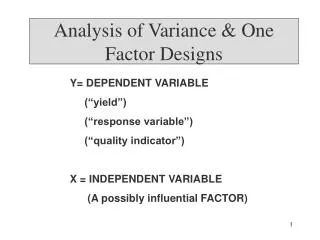
Analysis of Variance & One Factor Designs. Y= DEPENDENT VARIABLE (“yield”) (“response variable”) (“quality indicator”) X = INDEPENDENT VARIABLE (A possibly influential FACTOR) . OBJECTIVE: To determine the impact of X on Y Mathematical Model:

E N D
Analysis of Variance & One Factor Designs Y= DEPENDENT VARIABLE (“yield”) (“response variable”) (“quality indicator”) X = INDEPENDENT VARIABLE (A possibly influential FACTOR)
OBJECTIVE: To determine the impact of X on Y Mathematical Model: Y = f (x, ) , where = (impact of) all factors other than X Ex: Y = Battery Life (hours) X = Brand of Battery = Many other factors (possibly, some we’re unaware of)
StatisticalModel (Brand is, of course, represented as “categorical”) “LEVEL” OF BRAND 1 2 • • • • • • • • C 1 2 • • • • R Y11 Y12 • • • • • • •Y1c Yij = + j + ij i = 1, . . . . . , R j = 1, . . . . . , C Y21 • • • • • • YRI • • • • • Yij YRc • • • • • • • •
Where = OVERALL AVERAGE j = index for FACTOR (Brand) LEVEL i= index for “replication” j = Differential effect (response) associated with jth level of X and ij = “noise” or “error” associated with the (particular) (i,j)th data value. Let mj = AVERAGE associated with jth level of X tj = mj – m and m= AVERAGE of mj .
Yij = + j + ij By definition, j = 0 C j=1 The experiment produces R x C Yij data values. The analysis produces estimates of ,c. (We can then get estimates of the ij by subtraction).
2 3 C 1 • • • • • Y11 Y12 • • • • • •Y1c •••• Y21 • • • • YRI YRc • • • • • • • • • • • • (Y• j) • • Y• c Y• 1 Y• 2 Y•1, Y•2, etc., are Column Means
Y• • = Y• j /C = “GRAND MEAN” (assuming same # data points in each column) (otherwise, Y• • = mean of all the data) c j=1
MODEL: Yij = + j + ij Y• • estimates Y • j - Y • • estimatesj (= mj – m) (for all j) These estimates are based on Gauss’ (1796) PRINCIPLE OF LEAST SQUARES and (I would argue) on COMMON SENSE
MODEL: Yij = + j + ij If you insert the estimates into the MODEL, (1) Yij = Y • • + (Y•j - Y • • ) + ij. < it follows that our estimate of ij is (2) ij = Yij - Y•j <
Then, Yij = Y• • + (Y• j - Y• • ) + ( Yij - Y• j) or, (Yij - Y• • ) = (Y•j - Y• •) + (Yij - Y•j ) { { { (3) Variability in Y associated with all other factors Variability in Y associated with X TOTAL VARIABILITY in Y + =
If you square both sides of (3), and double sum both sides (over i and j), you get, [after some unpleasant algebra, but lots of terms which “cancel”] {{ C C R C R (Yij - Y• • )2 = R • (Y•j - Y• •)2 + (Yij - Y•j)2 { j=1 j=1 i=1 j=1 i=1 ( SSW (SSE) SUM OF SQUARES WITHIN COLUMNS TSS TOTAL SUM OF SQUARES SSBC SUM OF SQUARES BETWEEN COLUMNS + + = = ( ( ( ( (
ANOVA TABLE SOURCE OF VARIABILITY Mean square (M.S.) SSQ DF Between Columns (due to brand) SSBC SSBC C - 1 = MSBC C - 1 Within Columns (due to error) SSW MSW = (R - 1) • C SSW (R-1)•C TOTAL TSS RC -1
1 2 3 4 5 6 7 8 1.8 4.2 8.6 7.0 4.2 4.2 7.8 9.0 5.0 5.4 4.6 5.0 7.8 4.2 7.0 7.4 1.0 4.2 4.2 9.0 6.6 5.4 9.8 5.8 5.8 2.6 4.6 5.8 7.0 6.2 4.6 8.2 7.4 Example: Y = LIFETIME (HOURS) BRAND 3 replications per level SSBC = 3 ( [2.6 - 5.8]2 + [4.6 - 5.8] 2+ • • • + [7.4 - 5.8]2) = 3 (23.04) = 69.12
SSW = (1.8 - 2.6)2 = .64 (4.2 - 4.6)2 =.16 (9.0 -7.4)2 = 2.56 (5.0 - 2.6)2 = 5.76 (5.4 - 4.6)2= .64 • • • • (7.4 - 7.4)2 = 0 (1.0 - 2.6)2 = 2.56 (4.2 - 4.6)2= .16 (5.8 - 7.4)2 = 2.56 8.96 .96 5.12 Total of (8.96 + .96 + • • • • • • + 5.12), SSW = 46.72
ANOVA TABLE Source of Variability df M.S. SSQ 7 = 8 - 1 69.12 BRAND 9.87 ERROR 2.92 16 = 2 (8) 46.72 TOTAL 115.84 23 = (3 • 8) -1
We can show: “VCOL” { E (MSBC) = 2+ MEASURE OF DIFFERENCES AMONG COLUMN MEANS ( R ( • (j - )2 { C-1 j E (MSW) = 2 (Assuming each Yij has (constant) standard deviation, ) (More about assumptions, Later)
E ( MSBC ) = 2 +VCOL E ( MSW) = 2 This suggests that There’s some evidence of non-zero VCOL, or “level of X affects Y” if MSBC > 1 , MSW if MSBC No evidence that VCOL > 0, or that “level of X affects Y” < 1 , MSW
With HO: Level of X has no impact on Y HI: Level of X does have impact on Y, We need MSBC > > 1 MSW to reject HO.
More Formally, HO: 1 = 2 = • • • c = 0 HI: not all j = 0 OR (All column means are equal) HO: 1 = 2 = • • • • c HI: not all j are EQUAL
The probability Law of MSBC = “Fcalc” , is MSW The F - distribution with (C-1, (R-1)C) degrees of freedom Assuming HO true. C = Table Value
In our problem: ANOVA TABLE Source of Variability M.S. Fcalc SSQ df 7 69.12 BRAND 9.87 3.38 ERROR 2.92 = 9.87 2.92 16 46.72
F table coming up = .05 C = 2.66 3.38 (7,16 DF)
Hence, at = .05, Reject Ho . (i.e., Conclude that level of BRAND does have an impact on battery lifetime.)
SPSS/MINITAB INPUT VAR001 VAR002 1.8 1 5.0 1 1.0 1 4.2 2 5.4 2 4.2 2 . . . . . . 9.0 8 7.4 8 5.8 8
ONE FACTOR ANOVA (MINITAB) MINITAB: STAT>>ANOVA>>ONE-WAY Analysis of Variance for life Source DF SS MS F P brand 7 69.12 9.87 3.38 0.021 Error 16 46.72 2.92 Total 23 115.84
EXAMPLE: MORTARThe tension bond strength of cement mortar is an important characteristic of the product. An engineer is interested in comparing the strength of a modified formulation in which polymer latex emulsions have been added during mixing to the strength of the unmodified mortar. The experimenter has collected 10 observations on strength for the modified formulation and another 10 observations for the unmodified formulation.
Modified Unmodified16.85 17.5016.40 17.6317.21 18.2516.35 18.0016.52 17.8617.04 17.7516.96 18.2217.15 17.9016.59 17.9616.57 18.15Modified Unmodified16.85 17.5016.40 17.6317.21 18.2516.35 18.0016.52 17.8617.04 17.7516.96 18.2217.15 17.9016.59 17.9616.57 18.15
One-way ANOVA: strength versus type (Minitab)Analysis of Variance for strengthSource DF SS MS F Ptype 1 6.7048 6.7048 82.98 0.000Error 18 1.4544 0.0808Total 19 8.1592
Assumptions Basically, the same as in Regression analysis: MODEL: Yij = + j + ij 1.) the ij are indep. random variables 2.) Each ij is Normally Distributed E(ij) = 0 for all i, j 3.) 2(ij) = constant for all i, j Run order plot Normality plot Residual plot
Diagnosis: Normality • The points on the normality plot must more or less follow a line to claim “normal distributed”. • There are statistic tests to verify it scientifically. • The ANOVA method we learn here is not sensitive to the normality assumption. That is, a mild departure from the normal distribution will not change our conclusions much. Normality plot: normal scores vs. residuals
Diagnosis: Constant Variances • The points on the residual plot must be more or less within a horizontal band to claim “constant variances”. • There are statistic tests to verify it scientifically. • The ANOVA method we learn here is not sensitive to the constant variances assumption. That is, slightly different variances within groups will not change our conclusions much. Residual plot: fitted values vs. residuals
Diagnosis: Randomness/Independence • The run order plot must show no “systematic” patterns to claim “randomness”. • There are statistic tests to verify it scientifically. • The ANOVA method is sensitive to the constant variances assumption. That is, a little level of dependence between data points will change our conclusions a lot. Run order plot: order vs. residuals
This assumes a “fixed model”:Inherent interest in the specificlevels of the factors under study - there’s no direct interest in extrapolating to other levels - inference will be limited to levels that appear in the experiment. Experimenter selects the levels If a “random model”: Levels in experiment randomly selected from a population of such levels, and inference is to be made about the entire population of levels. Then, besides assumptions 1 to 3, there is another assumption: 4) a) the tj are independent random variables which are normally distributed with constant variance b) the tj and eij are independent
With these assumptions, the estimates (Y.. and the Y• j ) are “Maximum likelihood estimates”(a statistical notion which could be thought of as “efficiency” [“most likely value”]), and, more directly relevant: The “Conventional” F- and t- tests are applicable (VALID) for a variety of hypothesis testing and confidence interval computations.
KRUSKAL - WALLIS TEST (Non - Parametric Alternative) HO: The probability distributions are identical for each level of the factor HI: Not all the distributions are the same
Brand ABC 32 32 28 30 32 21 30 26 15 29 26 15 26 22 14 23 20 14 20 19 14 19 16 11 18 14 9 12 14 8 BATTERY LIFETIME (hours) (each column rank ordered, for simplicity) Mean: 23.9 22.1 14.9 (here, irrelevant!!)
HO: no difference in distribution among the three brands with respect to battery lifetime HI: At least one of the 3 brands differs in distribution from the others with respect to lifetime
Ranks Brand ABC 32 (29) 32 (29) 28 (24) 30 (26.5) 32 (29) 21 (18) 30 (26.5) 26 (22) 15 (10.5) 29 (25) 26 (22) 15 (10.5) 26 (22) 22 (19) 14 (7) 23 (20) 20 (16.5) 14 (7) 20 (16.5) 19 (14.5) 14 (7) 19 (14.5) 16 (12) 11 (3) 18 (13) 14 (7) 9 (2) 12 (4) 14 (7) 8 (1) T1 = 197T2 = 178 T3 = 90 n1 = 10 n2 = 10 n3 = 10
TEST STATISTIC: K 12 • (Tj2/nj ) - 3 (N + 1) H = N (N + 1) j = 1 nj = # data values in column j N = nj K = # Columns (levels) Tj = SUM OF RANKS OF DATA ON COL j When all DATA COMBINED (There is a slight adjustment in the formula as a function of the number of ties in rank.) K j = 1