Download
1 / 33
330 likes | 554 Views
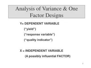
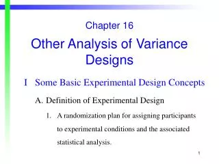
Other Analysis of Variance Designs. Chapter 15. Chapter Topics. Basic Experimental Design Concepts Defining Experimental Design Controlling Nuisance Variation The Randomized Block and Completely Randomized Factorial Designs Model Equation Computational Formulae and Procedures Assumptions

E N D
Other Analysis of Variance Designs Chapter 15
Chapter Topics • Basic Experimental Design Concepts • Defining Experimental Design • Controlling Nuisance Variation • The Randomized Block and Completely Randomized Factorial Designs • Model Equation • Computational Formulae and Procedures • Assumptions • Interactions • Multiple Comparison Procedures • Practical Significance
Experimental Design Concepts • Defining Experimental Design • “Refers to a randomization plan for assigning participants to experimental conditions and the statistical analysis associated with the plan” • We are going to discuss two designs: • Randomized Block Design • One treatment with two or more levels • Uses dependent samples • Usually more powerful than a Completely Randomized Design • Completely Randomized Factorial Design • Two or more treatments, each with two or more levels • Nuisance Variation • Any variation in the dependent variable systematically attributable to sources other than the independent variable.
Controlling Nuisance Variation • Three experimental approaches to controlling • Hold the nuisance variable constant • Use random sampling / random assignment • Include the nuisance variable as a variable in the experiment • Involves forming blocks of participants • Participants within a block are more homogeneous with respect to the nuisance variable than those in different blocks • Criteria for Blocking • Any variable correlated with the dependent variable other than the independent variable is a candidate to be a blocking variable • Four procedures • Repeated Measures • Participant Matching • Identical twins / littermates • Blocks matched by mutual selection
The Randomized Block Design • Linear Model Equation for a Score • Given by • The above parameters are generally unknown, but they can be estimated from sample data as follows: The Grand Mean The Treatment Effect The Block Effect The Error Effect
The Randomized Block Design (continued) • Interpreting the parameters • is the score for the person in the block and the population • is the grand mean of all scores in an experiment • is the effect of the population on this subject’s score • is the effect of the block on this subject’s score • is the random error effect on this subject’s score
The Randomized Block Design (continued) • In the RB-p design, we have two different omnibus null hypotheses we can test. • Equality of population treatment means • Equality of population block means
The Randomized Block Design (continued) • For this design, we are going to have four terms for sums of squares: • SSTO • Sums of Squares Total • Measures total variability among scores in an experiment • SSA • Sums of Squares Between Treatments • Measures variability between treatment levels • SSBL • Sums of Squares Within Blocks • Measures variability within blocks • SSRES • Sums of Squares Residual • Measure of “error” variability
The Randomized Block Design (continued) df=np-1 Completely Randomized Design df=p-1 df=p(n-1) Randomized Block Design df=n-1 df=(n-1)(p-1) df=p-1
The Randomized Block Design (continued) This is just another name for the total sample variance! This is the average variability between treatment levels. This is the average variability between blocks. This is the average “error” variability.
The Randomized Block Design (continued) • Just like in the CR-p design, in the RB-p design, what we want as researchers is for our “treatment levels” to account for more variation than does random error. • This design (and all designs) also uses the F statistic • Recall from previous chapters that the F statistic is defined as the ratio of two independent variances. • MSA and MSRES are both measures of variance, and they are independent of one another as are MSBL and MSRES. • Forming a ratio for each of these pairs yields two F statistics. Block Variable Test Treatment A Test
Computations in an RB-4 Design • We have computational formula for all of the sums of squares, and they are given by:
Computations in an RB-4 Design (continued) • Using the same data as we used in the CR-p design but modified to include blocks, we will compute these numbers Completely Randomized Design Randomized Block Design
Computations in an RB-4 Design (continued) • We compute the sums of squares as follows:
Computations in an RB-4 Design (continued) • We use these numbers to begin our ANOVA table
Computations in an RB-4 Design (continued) • This tests the hypothesis that the population treatment means are equal • If our computed F exceeds this number, we reject the null hypothesis. • It does, so we reject the null. • If the p-value is less than alpha, we reject the null • It is, so we reject Reject p-value a=.05 0 F3,21 F.05, 3, 21=3.07 F = 11.83
Computations in an RB-4 Design (continued) • This tests the hypotheses that the population means for the blocks are equal • Procedure is exactly the same as for testing the other hypothesis, but our df has changed! Reject p-value a=.05 0 F7,21 F.05, 7, 21=2.49 F = 3.31
Computations in an RB-4 Design (continued) • Analyze | Fit Model | Measurement in Y box (Continuous) | Grouping Variable AND Blocking Variable in “Effects” Box (Nominal) | • Different JMP procedure! • Output will be a little different than we’re used to . . .
Issues with an RB-p Design • In this example, we rejected both omnibus null hypotheses • The RB-p design can be more powerful than the CR-p design if . . . • . . . we selected a useful nuisance variable and matched participants effectively • What does “effectively” mean? • Nuisance variation should account for an appreciable portion of previously unexplained variation • The RB-p design can be less powerful than the CR-p design if . . . • . . . the loss in error df is not offset by a substantial decrease in error sums of squares
More on the RB-p Design • Multiple Comparison Procedures • These are the same as in a CR-p design with one exception: • MSRES is used instead of MSWG • Practical Significance • Similar measures, but in an RB-p design, we need a “partial” measure • Partial Omega-Squared • Measures the strength of association between the dependent variable and the treatment level • Values are interpreted the same as before • Cohen’s g
More on the RB-p Design (continued) • Assumptions • The model equation reflects all the sources of variation that affect each score • The blocks represent a random sample from the population of blocks. • The block effects are normally distributed and the variance of each block population is equal • The block effects are independent of each other and of other effects in the model equation • **The population variances of differences for all pairs of treatment levels are homogeneous • The error effects are normally distributed, and the variances of the error effects are homogeneous • The error effects are independent of one another and of other effects in the model equation
The CRF-pq Design • Factorial Design – two or more treatments • Treatment Combination – the combinations of conditions to which a participant is simultaneously exposed • Completely Crossed – each level of one treatment occurs with each level of another treatment • Partially Crossed – each level of one treatment occurs only with some levels of another treatment • Linear Model Equation
The CRF-pq Design (continued) The Grand Mean Treatment A Effect Treatment B Effect AB Interaction Effect The Error Effect
Interactions equal zero The CRF-pq Design (continued) • In the CRF-pq design, we have three different omnibus null hypotheses we can test. • Equality of population means for treatment A • Equality of population means for treatment B • Treatments A and B do not interact
Computations in a CRF-22 Design • Problem: Recall the PPA Example. Restaurant management is interested in determining whether average PPA differs across whether or not patrons consume alcohol in addition to whether or not it differs across gender. • There are two treatment levels here • Whether or not patrons consume alcohol – Two levels • Gender – Two levels (Male and Female) • First, we need to check to make sure the populations of treatment combinations are symmetric • This is done by obtaining several box-plots, one for each treatment combination, and placing them one above the other
Computations in a CRF-22 Design (continued) • We compute the sums of squares as follows:
Computations in a CRF-22 Design (continued) • We use these numbers to begin our ANOVA table
Computations in a CRF-22 Design (continued) • Interactions • The tests indicate that there is no interaction between gender and whether or not participants consume alcohol • In other words, differences in levels of one treatment are not different at two or more levels of the other treatment • The difference between men and women is essentially the same across ethnicities
Computations in a CRF-22 Design (continued) • Interactions • The lines on the previous graph were relatively parallel; this indicates no interaction • If the lines on the graph are non-parallel for some portion of the line, we have interaction.
Computations in a CRF-22 Design (continued) • This tests the hypotheses that the population means for treatment B are equal • Procedure is exactly the same for testing the other hypothesis, but our df may change! Reject p-value a=.05 0 F1,118 F.05, 1, 118=3.92 F = 9.78
Practical Significance in a CRF-pq Design • Practical Significance • “Partial” measures are used as in the RB-p case. • Partial Omega-Squared • Measures the strength of association between the dependent variable and the treatment level • For Treatment A . . . • For Treatment B . . . • There is also one for AxB interaction, computed similarly • Values are interpreted the same as before • Cohen’s g
CRF-pq Miscellanea • Multiple Comparison Procedures are the same as in the CR-p and RB-p designs • Assumptions with the CRF-pq Design • The model equation reflects all the sources of variation that affect each score • Participants are random samples from the respective populations or the participants have been randomly assigned to the treatment combinations • The population for each of the treatment combinations is normally distributed • The variance of each of the pq treatment combinations are equal
Chapter Highlights • We have developed a definition of experimental design through two designs, each of which are slightly more complex than the CR-p design • Randomized Block • Isolates a nuisance variable in hopes of reducing error variance • Completely Randomized Factorial • Allows the researcher to test two treatments and the interaction between the treatments • Each has the potential to have of greater power than the CR-p design • There are many, many more designs out there. We have introduced the three which are most common.