Download
1 / 34
340 likes | 738 Views
2. Pipeline terminology. The pipeline depth is the number of stages

E N D
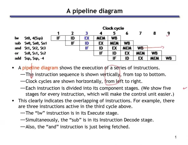
1. 1 A pipeline diagram A pipeline diagram shows the execution of a series of instructions.
The instruction sequence is shown vertically, from top to bottom.
Clock cycles are shown horizontally, from left to right.
Each instruction is divided into its component stages. (We show five stages for every instruction, which will make the control unit easier.)
This clearly indicates the overlapping of instructions. For example, there are three instructions active in the third cycle above.
The �lw� instruction is in its Execute stage.
Simultaneously, the �sub� is in its Instruction Decode stage.
Also, the �and� instruction is just being fetched.
2. 2 Pipeline terminology The pipeline depth is the number of stages�in this case, five.
In the first four cycles here, the pipeline is filling, since there are unused functional units.
In cycle 5, the pipeline is full. Five instructions are being executed simultaneously, so all hardware units are in use.
In cycles 6-9, the pipeline is emptying.
3. 3 Pipelined datapath and control Now we�ll see a basic implementation of a pipelined processor.
The datapath and control unit share similarities with both the single-cycle and multicycle implementations that we already saw.
An example execution highlights important pipelining concepts.
In future lectures, we�ll discuss several complications of pipelining that we�re hiding from you for now.
4. 4 Pipelining concepts A pipelined processor allows multiple instructions to execute at once, and each instruction uses a different functional unit in the datapath.
This increases throughput, so programs can run faster.
One instruction can finish executing on every clock cycle, and simpler stages also lead to shorter cycle times.
5. 5 Pipelined Datapath The whole point of pipelining is to allow multiple instructions to execute at the same time.
We may need to perform several operations in the same cycle.
Increment the PC and add registers at the same time.
Fetch one instruction while another one reads or writes data.
Thus, like the single-cycle datapath, a pipelined processor will need to duplicate hardware elements that are needed several times in the same clock cycle.
6. 6 We need only one register file to support both the ID and WB stages.
Reads and writes go to separate ports on the register file.
Writes occur in the first half of the cycle, reads occur in the second half.
One register file is enough
7. 7 Single-cycle datapath, slightly rearranged
8. 8 What�s been changed? Almost nothing! This is equivalent to the original single-cycle datapath.
There are separate memories for instructions and data.
There are two adders for PC-based computations and one ALU.
The control signals are the same.
Only some cosmetic changes were made to make the diagram smaller.
A few labels are missing, and the muxes are smaller.
The data memory has only one Address input. The actual memory operation can be determined from the MemRead and MemWrite control signals.
The datapath components have also been moved around in preparation for adding pipeline registers.
9. 9 Multiple cycles In pipelining, we also divide instruction execution into multiple cycles.
Information computed during one cycle may be needed in a later cycle.
The instruction read in the IF stage determines which registers are fetched in the ID stage, what constant is used for the EX stage, and what the destination register is for WB.
The registers read in ID are used in the EX and/or MEM stages.
The ALU output produced in the EX stage is an effective address for the MEM stage or a result for the WB stage.
We added several intermediate registers to the multicycle datapath to preserve information between stages, as highlighted on the next slide.
10. 10 Registers added to the multi-cycle
11. 11 Pipeline registers We�ll add intermediate registers to our pipelined datapath too.
There�s a lot of information to save, however. We�ll simplify our diagrams by drawing just one big pipeline register between each stage.
The registers are named for the stages they connect.
IF/ID ID/EX EX/MEM MEM/WB
No register is needed after the WB stage, because after WB the instruction is done.
12. 12 Pipelined datapath
13. 13 Propagating values forward Any data values required in later stages must be propagated through the pipeline registers.
The most extreme example is the destination register.
The rd field of the instruction word, retrieved in the first stage (IF), determines the destination register. But that register isn�t updated until the fifth stage (WB).
Thus, the rd field must be passed through all of the pipeline stages, as shown in red on the next slide.
Why can�t we keep a single instruction register like we did in the multi-cycle data-path?
14. 14 The destination register
15. 15 What about control signals? The control signals are generated in the same way as in the single-cycle processor�after an instruction is fetched, the processor decodes it and produces the appropriate control values.
But just like before, some of the control signals will not be needed until some later stage and clock cycle.
These signals must be propagated through the pipeline until they reach the appropriate stage. We can just pass them in the pipeline registers, along with the other data.
Control signals can be categorized by the pipeline stage that uses them.
16. 16 Pipelined datapath and control
17. 17 What about control signals? The control signals are generated in the same way as in the single-cycle processor�after an instruction is fetched, the processor decodes it and produces the appropriate control values.
But just like before, some of the control signals will not be needed until some later stage and clock cycle.
These signals must be propagated through the pipeline until they reach the appropriate stage. We can just pass them in the pipeline registers, along with the other data.
Control signals can be categorized by the pipeline stage that uses them.
18. 18 Pipelined datapath and control
19. 19 Notes about the diagram The control signals are grouped together in the pipeline registers, just to make the diagram a little clearer.
Not all of the registers have a write enable signal.
Because the datapath fetches one instruction per cycle, the PC must also be updated on each clock cycle. Including a write enable for the PC would be redundant.
Similarly, the pipeline registers are also written on every cycle, so no explicit write signals are needed.
20. 20 Here�s a sample sequence of instructions to execute.
1000: lw $8, 4($29)
1004: sub $2, $4, $5
1008: and $9, $10, $11
1012: or $16, $17, $18
1016: add $13, $14, $0
We�ll make some assumptions, just so we can show actual data values.
Each register contains its number plus 100. For instance, register $8 contains 108, register $29 contains 129, and so forth.
Every data memory location contains 99.
Our pipeline diagrams will follow some conventions.
An X indicates values that aren�t important, like the constant field of an R-type instruction.
Question marks ??? indicate values we don�t know, usually resulting from instructions coming before and after the ones in our example. An example execution sequence
21. 21 Cycle 1 (filling)
22. 22 Cycle 2
23. 23 Cycle 3
24. 24 Cycle 4
25. 25 Cycle 5 (full)
26. 26 Cycle 6 (emptying)
27. 27 Cycle 7
28. 28 Cycle 8
29. 29 Cycle 9
30. 30 That�s a lot of diagrams there
Compare the last nine slides with the pipeline diagram above.
You can see how instruction executions are overlapped.
Each functional unit is used by a different instruction in each cycle.
The pipeline registers save control and data values generated in previous clock cycles for later use.
When the pipeline is full in clock cycle 5, all of the hardware units are utilized. This is the ideal situation, and what makes pipelined processors so fast.
Try to understand this example or the similar one in the book at the end of Section 6.3.
31. 31 Performance Revisited Assuming the following functional unit latencies:
What is the cycle time of a single-cycle implementation?
What is its throughput?
What is the cycle time of a ideal pipelined implementation?
What is its steady-state throughput?
How much faster is pipelining?
32. 32 Ideal speedup In our pipeline, we can execute up to five instructions simultaneously.
This implies that the maximum speedup is 5 times.
In general, the ideal speedup equals the pipeline depth.
Why was our speedup on the previous slide �only� 4 times?
The pipeline stages are imbalanced: a register file and ALU operations can be done in 2ns, but we must stretch that out to 3ns to keep the ID, EX, and WB stages synchronized with IF and MEM.
Balancing the stages is one of the many hard parts in designing a pipelined processor.
33. 33 The pipelining paradox Pipelining does not improve the execution time of any single instruction. Each instruction here actually takes longer to execute than in a single-cycle datapath (15ns vs. 12ns)!
Instead, pipelining increases the throughput, or the amount of work done per unit time. Here, several instructions are executed together in each clock cycle.
The result is improved execution time for a sequence of instructions, such as an entire program.
34. 34 Instruction set architectures and pipelining The MIPS instruction set was designed especially for easy pipelining.
All instructions are 32-bits long, so the instruction fetch stage just needs to read one word on every clock cycle.
Fields are in the same position in different instruction formats�the opcode is always the first six bits, rs is the next five bits, etc. This makes things easy for the ID stage.
MIPS is a register-to-register architecture, so arithmetic operations cannot contain memory references. This keeps the pipeline shorter and simpler.
Pipelining is harder for older, more complex instruction sets.
If different instructions had different lengths or formats, the fetch and decode stages would need extra time to determine the actual length of each instruction and the position of the fields.
With memory-to-memory instructions, additional pipeline stages may be needed to compute effective addresses and read memory before the EX stage.
35. 35 Summary The pipelined datapath combines ideas from the single and multicycle processors that we saw earlier.
It uses multiple memories and ALUs.
Instruction execution is split into several stages.
Pipeline registers propagate data and control values to later stages.
The MIPS instruction set architecture supports pipelining with uniform instruction formats and simple addressing modes.
Next lecture, we�ll start talking about Hazards.