Download

1 / 0
0 likes | 125 Views
Particle Filters++ Pieter Abbeel UC Berkeley EECS Many slides adapted from Thrun , Burgard and Fox, Probabilistic Robotics. TexPoint fonts used in EMF. Read the TexPoint manual before you delete this box.: A A A A A A A A A A A A A.

E N D