Download
1 / 13
130 likes | 157 Views
This study focuses on optimizing photon discrimination efficiency in the CMS detector using moments variables. It investigates the effectiveness of various moment variables like MMAJ2 and MMIN2, Lateral moment LAT, and Pseudo-zernike moment PZM in distinguishing between photon and pi0 events. The analysis compares different versions of CMSSW_3_1_2 and evaluates the performance of classifiers like Fisher, MLP, LikelihoodD, PDERS, RuleFit, HMatrix, BDT, CutsGA, and Likelihood to enhance signal efficiency and background rejection. The study sheds light on overtraining checks and presents results on signal efficiency versus background efficiency for each method. Furthermore, it delves into the definition and significance of moments variables in discriminating between different particle events.

E N D
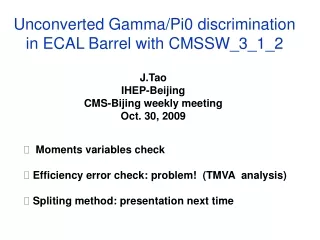
Unconverted Gamma/Pi0 discrimination in ECAL Barrel with CMSSW_3_1_2 J.Tao IHEP-Beijing CMS-Bijing weekly meeting Oct. 30, 2009 • Moments variables check • Efficiency error check: problem! (TMVA analysis) • Spliting method: presentation next time
Moments variable • Second-order moments: MMAJ2 & MMIN2 • Lateral moment LAT • Pseudo-zernike moment PZM • LAT& PZM can be obtained from the default shower shape variables from SW Dataformat. • MMAJ2 & MMIN2 were calculated by myself
Comparision: LAT & PZM • Samples: Single , π0 → samples with E from 30GeV to 70GeV • Unconverted case in Barrel CMSSW_3_1_2 CMS AN-2008/075 Version ? : peak~0.11 : peak~0.15 : peak~0.81 : peak~0.86 • The distributions are some different for diferent version
Comparision: MMAJ2 & MMIN2 Distribution of the average value of MMin2 for and π0, as a function of EST MMAJ2 : peak~0.25 : peak~0.35 Distribution of the average value of MMAJ2 for and π0, as a function of EST
EST CMS AN-2008/075 we can compute an estimate of (in the hypothesis of a π0 ) by replacing L(0 ) and α(E1,E2) with the reconstructed quantities dened in Eq. 2 and 4:
EST v.s. reco. E CMS AN-2008/075 Pi0 sample CMSSW_3_1_2: Pi0 sample • 0.5 < _EST < 0.8 cm; • 0.8 < _EST < 1 cm; • 1.0 < _EST < 1.2 cm
Results with Moments variables: 0.8 < _EST < 1 cm For MMAJ2 only: ~29% Pi0 rejection 47.0% 0.8 < _EST < 1 cm 0.8 < _EST < 1 cm Efciency of photon identication vs π0 rejection for MMAJ2, LAT and PZM. Much different result!
Efficiency error check • Smooth background rejection versus signal efficiency curve: (from cut on classifier output) • Problem: how to get the efficienfy error at each efficiency point?
Evaluating the Classifiers (taken from TMVA output…) Evaluation results ranked by best signal efficiency and purity (area) ------------------------------------------------------------------------------ MVA Signal efficiency at bkg eff. (error): | Sepa- Signifi- Methods: @B=0.01 @B=0.10 @B=0.30 Area | ration: cance: ------------------------------------------------------------------------------ Fisher : 0.268(03) 0.653(03) 0.873(02) 0.882 | 0.444 1.189 MLP : 0.266(03) 0.656(03) 0.873(02) 0.882 | 0.444 1.260 LikelihoodD : 0.259(03) 0.649(03) 0.871(02) 0.880 | 0.441 1.251 PDERS : 0.223(03) 0.628(03) 0.861(02) 0.870 | 0.417 1.192 RuleFit : 0.196(03) 0.607(03) 0.845(02) 0.859 | 0.390 1.092 HMatrix : 0.058(01) 0.622(03) 0.868(02) 0.855 | 0.410 1.093 BDT : 0.154(02) 0.594(04) 0.838(03) 0.852 | 0.380 1.099 CutsGA : 0.109(02) 1.000(00) 0.717(03) 0.784 | 0.000 0.000 Likelihood : 0.086(02) 0.387(03) 0.677(03) 0.757 | 0.199 0.682 ------------------------------------------------------------------------------ Testing efficiency compared to training efficiency (overtraining check) ------------------------------------------------------------------------------ MVA Signal efficiency: from test sample (from traing sample) Methods: @B=0.01 @B=0.10 @B=0.30 ------------------------------------------------------------------------------ Fisher : 0.268 (0.275) 0.653 (0.658) 0.873 (0.873) MLP : 0.266 (0.278) 0.656 (0.658) 0.873 (0.873) LikelihoodD : 0.259 (0.273) 0.649 (0.657) 0.871 (0.872) PDERS : 0.223 (0.389) 0.628 (0.691) 0.861 (0.881) RuleFit : 0.196 (0.198) 0.607 (0.616) 0.845 (0.848) HMatrix : 0.058 (0.060) 0.622 (0.623) 0.868 (0.868) BDT : 0.154 (0.268) 0.594 (0.736) 0.838 (0.911) CutsGA : 0.109 (0.123) 1.000 (0.424) 0.717 (0.715) Likelihood : 0.086 (0.092) 0.387 (0.379) 0.677 (0.677) ----------------------------------------------------------------------------- Better classifier
Moments variable 1 – second-order moments Distribution of energy deposit for π0 with = 6 cm, overlaid with the major (solid line) and minor(dotted line) axes. Distribution of the average value of MMAJ2 for and π0, as a function of EST Distribution of the average value of MMin2 for and π0, as a function of EST • Definition of monents of order n: where dMAJi (dMINi ) is the distance between the center of the i-th crystal and the major (minor) axis, expressed in terms of η, indices. • Major & minor axes, dened as the eigenvectors of the covariance matrix where N is the number of crystals in the cluster, i and i are the η, indices that identify the i-th crystal of the cluster and . The weight I (The eigenvalues are 1 and 2 in NN variables) • Moments with n > 2 are strongly correlated with second-order moments and therefore they are useless. • So MMAJ2 & MMIN2. In fact only MMAJ2 is powerful for the discrimination of /π0.
Moments variable 2 – Lateral moment LAT • Definition of LAT: where E1 and E2 are the energies of the two most energetic crystals of the cluster. • Expression of r2: • where ~ri is the radius vector of the i-th crystal, ~r is the radius vector of the cluster centroid and rM is the Moliere radius of the electromagnetic calorimeter (2.2 cm for PbWO4). Note that the two most energetic crystals are left out of the sum in this Eq. • Distribution of LAT
Moments variable 3 – Pseudo-zernike moment • The pseudo-Zernike moments Anm are dened as where n and m are two integers. • The complex polynomials Vnm*(i,i), expressed in polar coordinates, are dened as • The cluster shape viable PZM used in the analysis is computed as i. e. the norm of the A20 moment. • Distribution of PZM