Download
1 / 35
350 likes | 440 Views
This study delves into the localization effect in ionospheric conductivity on Aurora intensity by analyzing the feedback mechanism between Alfvén waves and ionosphere. The model explores the interaction of simple bouncing Alfvén waves between ionosphere and magnetosphere. Through various equations and models, the text examines the impact of ionospheric conductivity on the intensification and concentration of Aurora activities. Different cases are formulated to study incident wave behavior, considering parameters like electric field, energy loss, and wave reflection. The study highlights the influence of various factors on Aurora concentration and geomagnetic activities.

E N D
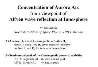
Concentration of Aurora Arc from viewpoint of Alfvén wave reflection at Ionosphere M.Yamauchi Swedish Institute of Space Physics (IRF), Kiruna (A) Aurora (J//) ÜÞ Geomagnetic activities (I^) Newell's work (low sP gives higher e- energy) but low I^ and E^ for in winter hemisphere (B) Semi-annual peak of the Geomagnetic (Aurora) activities Kp & nightside AL Þsemi-annual peak AU & dayside AL Þannual peak
Ideally, we have to examine all aspects of * Solar Wind Þ Magnetosphere * Magnetospheric Response * Magnetosphere Þ Ionosphere * Magnetosphere-Ionosphere System * Ionospheric Response * Role of Ground and Cavity Mode But, ONLY the effect of Ionospheric conductivity (sP) is considered today (Sorry, all the other aspects are ignored). What kind of ionosphericsPeffect has been overlooked?
(A) Localization/intensification of J// & I^ by low SP High concentration of J// when ∆SP/SP is high, i.e., when SP is low for given ∆SP through the positive feed-back between J// enhancement and SP enhancement Study interaction between Alfvén Wave ÜÞ Ionosphere. • Use a simple bouncing Alfvén wave model between the ionosphere and the magnetosphere [Sato and Iijima 1980, Kan and Sun 1985]
Alfvén wave bouncing model (to study thelocalization effect) <step 1> MHD Alfvén wave µ dj/dt = -Ñ´Ñ´ E dE/dt = B0´ (j´B0) / r + plane wave approximation ( d/dt = ±VA d/dz & Ñ ^·E^ = 0 ) µVAj^ = ±dE/dz ( where db/dz = µj^´z ) integrating over z, ∆I = ± SA∆E ∆b = ±∆E´z/VA where SA = 1/(µVA) sign (±) depends on propagation direction.
+ simple reflection model (incident, reflect, and transmitting) ∆Eincident + ∆Ereflect = total ∆E in the ionosphere = E^(new) -E^(old) ∆bincident + ∆breflect = total ∆b above the ionosphere or SA (∆Eincident- ∆Ereflect) = ∆I^ where ∆ is the stepwise change by the wave, E^ (and I^) are the ionospheric electric field and current. + ionospheric Ohm's law (hall current = B0´E direction) I^ = SPE^ + z ´SHE^ Jz = - ∫Ñ^·j^ dz
All together SA∆E^(new) + ∆I^(new) = 2 SA∆Eincident+SA∆E^(old) + ∆I^(old) or [SA+SP+(SHz ´)]∆E^ = 2 SA∆Eincident-[∆SP+(∆SHz ´)] E^(old) or [(SP+SA)2 + SH2]∆E^ = 2 SA [(SA+SP) - SHz ´] ∆Eincident - [(SA+SP)∆SP + SH∆SH + SA∆SHz ´] E^(old) ∆Ereflect = ∆E^- ∆Eincident E^(new) = ∆E^ + E^(old) J// = -Ñ^·I^ where J// > 0 means upward current (electron precipitation) in both hemisphere
<step 2> ∆SP model by precipitation • SP2= S02 + g J'// (J'//- Jthreshold) • SH / SP = constant • where • J'// = min (J// , Jsaturation) and J'// = 0 if J// < Jthreshold • Jsaturation = 1 µA/m2 is the maximum current density • Jthreshold = Jsaturation/10 is threshold current density • g ≈ (14 SA / Jsaturation)2 ≈ [ (10 mho)/(1 µA/m2) ]2 • In the normalized equation (to electric field in [mV/m]): • J*saturation = 1.5 ~ 5 • J*threshold = 0.15 ~ 0.5 • (for L = 1000 ~ 2000 km, VA = 1000 ~ 2000 km/s) • E0 = 0.1 ~ 0.3 mV/m
<step 3> How to model "next" incident wave • We formulated three cases: simple reflection, forced constant convection, • and dissipating convection (a) Eincident= lEreflect • where -1 < l < +1 • (opposite hemisphere : l > 0) [cf. Kan and Sun, 1985] (b) Eincident=E0-E^ and ∆E0=- kI^· E^ where k = 0.01 ~0.1 represents the energy loss (l=-1 with finite convection) [cf. Sato and Iijima, 1980]
Range of the parameters • parameter range • H /P 0.1 ~ 2.5 • 0 / A 1 ~ 25 • Jthreshold / Jsaturation 0.1 • Jsaturation L/(A E0) 0.1 ~ 5 • E02/A2 0.1 ~ 5 • > 0 0.5 ~ 1.0 • < 0 - 0.5 ~ - 1.0 • A E0 0.0015 ~ 0.015 • ∆/L 0.01 ~ 0.08 Initial condition: ∆Eincident = E0 sin(2πX/L)
Ex Ix SP/SA J// • (a) Ein= lEref • J*sat = 1.5 • J*thre= 0.15 • E0 = 0.1 [mV/m] • SP/SA= 1, 5, 25 • SH/SP= 0.5 • l = 0.7
<step 4> Problem and limitation (1) Linear wave reflection model means IE is highest when the impedance matches (P =A), i.e., low P gives high local dissipationwhen P > A. But, observation = low potential drop for low P in winter. Þ ? (I simply do not know the answer) (2) There are many free parameters, we can get nearly any result by adjusting then. One must extract only common quntitative feature. (3) We need artificial diffusion for stability because the system is positive feedback. It is difficult to find physically correct mixing width. (4) Notes in 1-D (∂/∂y = 0) model: * Qc = dEx/dx gives only perpendicular potential field. * ∂Bz/∂t = ∂Ey/∂x is ignored * Modulation of source convection in Ey direction is ignored.
function Y = diffuse(A, Nx, loop, vcs) % smoothing subroutine A[1:Nx] --> Y[1:Nx] % (1) loop=0: no smoothing % (2) loop<0: averaging over |loop| length % (3) loop>0: 1-degree diffusion x loop times + averaging for i = 1:1:Nx; Y(i) = A(i); end; lp = fix(abs(loop)); if (loop == 0) else w2 = 2*lp + 2.0; for i = 1:1:Nx; for j = -lp:1:lp; ij = i + j; if (ij < 1) ij = ij + Nx; end; if (ij > Nx) ij = ij - Nx; end; Y(i) = Y(i) + A(ij); end; %for j Y(i) = Y(i) / w2; end; %for i end; %if loop if (loop > 0) for j = 1:1:lp; for i = 1:1:Nx; B(i)=Y(i); end; for i = 1:1:Nx; in = i - 1; ip = i + 1; if (in < 1) in = in + Nx; end; if (ip > Nx) ip = ip - Nx; end; Y(i) = vcs * ( B(ip) + B(in) - 2*B(i) ) + B(i); end; %for i end; %for j end; %if loop loop = SP loop/2 = Jz, ∆E^ , E^, J^
Ein= lEref , J*sat = 1.5 , J*thre= 0.15 , E0 = 0.1 [mV/m] SP/SA= 1 , SH/SP= 0.5 , l = 0.7 Ex Ix SP/SA J// Ave = 1~2% , 2~4% , 4~8% , 6~12% , 8~16%
(b) Ein=E0-E^, J*sat = 1.5 , J*thre= 0.15 , E0 = 0.1 [mV/m] SP/SA= 1 , SH/SP= 0.5 Ex Ix SP/SA J// Ave = 1~2% , 2~4% , 4~8% , 6~12% , 8~16%
Ex Ix SP/SA J// (a) Ein= lEref J*sat = 1.5 J*thre= 0.15 E0 = 0.1 [mV/m] SP/SA= 5 SH/SP= 0.5 l = 0.7, 1, -0.7
Ex Ey Ix Iy SP/SA J// • (a) Ein= lEref • J*sat = 1.5 • J*thre= 0.15 • E0 = 0.1 [mV/m] • SP/SA= 5 • SH/SP= 0.1, 0.5, 1.5 • l = 0.7 • No effect !
(b) Ein=E0-E^ ∆Ein=- kI^·E^ J*sat = 1.5 J*thre= 0.15 E0 = 0.1 [mV/m] SP/SA= 1, 5, 25 SH/SP= 0.5 k = 0.03 Ex Ix SP/SA J//
(b) Ein=E0-E^ (k = 0) J*sat = 1.5 J*thre= 0.15 E0 = 0.1 [mV/m] SP/SA= 1, 5, 25 SH/SP= 0.5 Ex Ix SP/SA J//
(b) Ein=E0-E^ ∆Ein=- kI^·E^ J*sat = 1.5 J*thre= 0.15 E0 = 0.1 [mV/m] SP/SA= 5 SH/SP= 0.5 k = 0.01, 0.03, 0.1 Ex Ix SP/SA J//
(b) Ein=E0-E^ ∆Ein=- kI^·E^ J*sat = 5 J*thre= 0.5 E0 = 0.3 [mV/m] SP/SA= 5 SH/SP= 0.5 k = 0.01, 0.03, 0.1 Ex Ix SP/SA J//
Summery of the bouncing wave model (1) Concentration (filamentation) of J// for low SP case is gerenrally found as long as J// exceeds threshold value. J// is higher for low SP than high SP for the same level of Ix (i.e., geomagnetic disturbance). (2) Conditions for filamentation is a complicated fuction of many factors: * SP / SA and SH / SA * magnetospheric "reflection" process * mixing (diffusion) width * relation between ∆SP and J// * Jsaturation and Jthreshold * amplitude of incident Alfvén wave (3) Ionospheric current (or ground ∆B) and J// density have only weak direct correlation.
(B) Decay of magnetospheric energy by sP of entire hemisphere High dissipation during winter through the summer hemisphere. Equinox converts convection energy to the aurora effectively. Calculate the accumulated input energy (e·t) for different seasons using a simple circuit model. e : instantaneous input energy eµsP. t : decay time of total energy t µ 1/∫N+SsP Þ Simply calculate e·t µsP / ∫N+SsP
Lat 90° 60° 90° 50° 90° 50° 90° 60° 90° 50° Solstice case 12 LT 18 LT 24 LT * Chapman a layer sPµ √cos(q) * Chapman b layer sPµ cos(q) where q is the solar zeneath angle 12 LT 18 LT 24 LT
Faint precipitation case Strong precipitation case Lat 90° 50° 90° 50° inc=23° inc=14° inc=5°
24 LT 22 LT 20 LT 18 LT 16 LT Result !
Faint precipitation case Strong precipitation case 24 LT 22 LT 20 LT 18 LT 16 LT
Summery of the simple circuit model (1) The semi-annual variation of the geomagnetic activity is reproduced from a very simple circuit model using conductivity effect (SP/∫N+SSP) only. (2) Semi-annual variation of SP/∫N+SSPis found in wide range of LT, and is most prominent at 60-70° latitude. (3) Since large activity corresponds to wide area of "decay" region (integral becomes wide), we expect that intensity of substorms for same input has more clearly semi-annual variation. Þ Need to examine the Kp dependence of the semi-annual variation to check Kp variation is consistent with the SP/∫N+SSP model.
axis = number of 3-hour periods during a 4-month period Each x represents 1-year data
(b) Ein=E0-E^ • ∆Ein=- kI^·E^ • J*sat = 1.5 • J*thre= 0.15 • E0 = 0.1 [mV/m] • SP/SA= 5 • SH/SP= 0.1, 0.5, 1.5 • k = 0.03 • No effect ! Ex Ey Ix Iy SP/SA J//
SP/SA= 5 SH/SP= 0.1, 0.5, 1.5 No effect !
Ex Ix SP/SA J// • (a) Ein= lEref • J*sat = 5 • J*thre= 0.5 • E0 = 0.3 [mV/m] • SP/SA= 1, 5, 25 • SH/SP= 0.5 • l = 0.7
(b) Ein=E0-E^ ∆Ein=- kI^·E^ J*sat = 5 J*thre= 0.5 E0 = 0.3 [mV/m] SP/SA= 1, 5, 25 SH/SP= 0.5 k = 0.03 Ex Ix SP/SA J//
(b) Ein=E0-E^ (k = 0) J*sat = 5 J*thre= 0.5 E0 = 0.3 [mV/m] SP/SA= 1, 5, 25 SH/SP= 0.5 Ex Ix SP/SA J//
Ex Ix SP/SA J// (a) Ein= lEref J*sat = 5 J*thre= 0.5 E0 = 0.3 [mV/m] SP/SA= 5 SH/SP= 0.5 l = 0.7, 1, -0.7