Getting Started

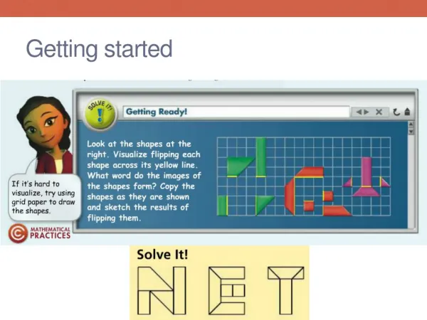
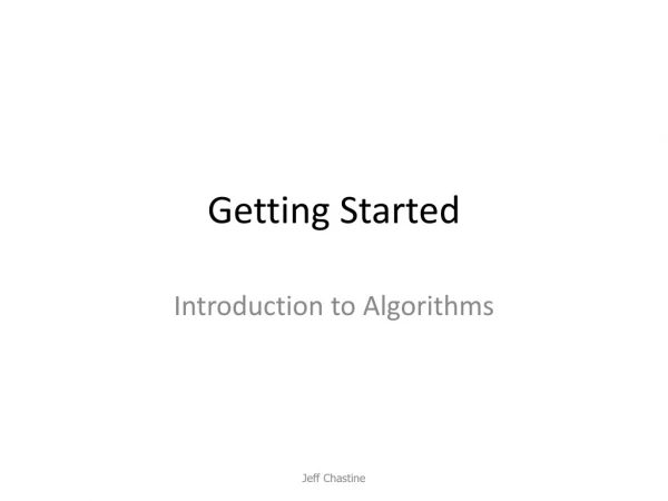
1. Getting Started Introduction to Algorithms Jeff Chastine

2. Hard to find Symbols in PPT • ƒßΘΟΣΦΩαβθωο‹›←→↔∑∞∫≠≤ ≥≈≡☺☻ Jeff Chastine

3. A Little Boy and His Teacher • A troublesome student (named Bob) was asked to sum the numbers between 1 and 100 in order to keep him busy. He came up with this formula: n n(n+1) ∑ i = 2 i=1 Why does this work? Jeff Chastine

4. When n = 10 1 2 3 4 5 6 7 8 9 10 5 4 3 2 1 1+10=11, 2+9=11, 3+8=11, etc… You do this n/2 times Jeff Chastine

5. Sorting Problem • Input: A sequence of n numbers<a1, a2, …, an> • Output: A permutation <a'1, a'2, …, a'n> of the original such that a'1 ≤ a'2 ≤ …≤ a'n • Sorting is fundamental to computer science, so we’ll be studying several different solutions to it Jeff Chastine

6. Insertion Sort • Uses two “hands” • Left – initially empty • Right – initially the original array • Move a card from the right hand to the left • Find the correct position by going from right to left (in the already sorted left hand) • We say that insertion sort is sorted in place (no additional memory needed) Jeff Chastine

7. Insertion Sort 1 for j ← 2 tolength[A] 2 dokey ← A[ j ] 3 // Insert A[ j ] into the sorted sequence A[ j – 1] 4 i ← j - 1 5 whilei > 0 and A[i] > key 6 doA[i+1] ← A[i] 7 i ← i - 1 8 A[i+1] ← key A =‹5, 2, 4, 6, 1, 3› Jeff Chastine

8. Correctness of Insertion Sort • We can use loop invariants: • Initialization – true prior to first iteration • Maintenance – remains true before the next iteration • Termination – remains true after the loop terminates • At the start of each iteration, the subarray A [1 .. j -1] is in sorted order Jeff Chastine

9. Correctness of Insertion Sort • Initialization: when j = 2, A [1 .. j – 1] holds a single element • Maintenance: inner loop moves elements to the right until the proper position is found. A[ j ] is inserted into the correct position • Termination: j = n + 1, which is beyond n Jeff Chastine

10. Analyzing Algorithms • Analyzing an algorithm usually means determining how much computational time is taken to solve a given problem • Input size usually means the number of items in the input (elements to be sorted, number of bits, number of nodes in a graph) • Running time is the number of primitive operations executed (and is device independent) Jeff Chastine

11. Analysis of Insertion Sort • Worst case: sorted in descending order (runs as a quadratic an2 + bn + c, you’ll see) • Best case scenario: numbers sorted in ascending order (linear function n) • Why? This loop won't have to run! 5 whilei > 0 and A[i] > key c5 6 doA[i+1] ← A[i] c6 7 i ← i - 1 c7 Jeff Chastine

12. Insertion Sort 1 for j ← 2 tolength[A] c1n 2 dokey ← A[ j ] c2n-1 3 // Insert … c3 n-1 4 i ← j - 1 c4n-1 5 whilei > 0 and A[i] > key c5∑ 6 doA[i+1] ← A[i] c6∑ 7 i ← i - 1 c7∑ 8 A[i+1] ← key c8 n-1 n tj j=2 n (tj - 1) j=2 n (tj - 1) j=2 Jeff Chastine

13. n Thanks Bob! → n(n+1) ∑ j = -1 2 j=2 T(n)= c1n + c2(n-1) + c4(n-1) + c5((n(n+1))/2-1) + c6((n(n-1))/2) + c7((n(n-1))/2) + c8 = (c5/2 + c6/2 + c7/2) n2 + (c1+c2+c4+c5/2-c6/2-c7/2+c8) n - (c2+c4+c5+c8) Jeff Chastine

14. Rate of Growth • The rate of growth is what we're interested in • Only consider leading term (other terms are insignificant, as you will see) • Also ignore leading term's coefficient a • Constants are less significant than rate of growth • Therefore, we say worst-case for insertion sort is Θ(n2) • What is the best case for this algorithm? • What about the average/expected case? Jeff Chastine

15. The Divide-and-Conquer Approach • These algorithms are recursive in structure • Call themselves with a subset of the given problem • Then combine solutions back together • Question: how to recursively fill in the screen? Jeff Chastine

16. MERGE SORT • Divide n-element array into two subsection of n/2 size • Conquer: sort the two subsections recursively using Merge Sort • Merge the sorted subarrays to produce sorted answer • Note: a unit of 1 is, by definition, sorted. Jeff Chastine

17. The Code MERGE-SORT (A, p, r) 1 ifp < r 2 thenq ←(p+r)/2 3 MERGE-SORT(A, p, q) 4 MERGE-SORT(A, q+1, r) 5 MERGE (A, p, q, r) Jeff Chastine

18. MERGE SORT(Divide) 5 2 4 6 1 3 2 6 5 2 4 6 1 3 2 6 5 2 4 6 1 3 2 6 5 2 4 6 1 3 2 6 Jeff Chastine

19. MERGE SORT(Merge – where the work’s done) 1 2 2 3 4 5 6 6 2 4 5 6 1 2 3 6 2 5 4 6 1 3 2 6 5 2 4 6 1 3 2 6 Jeff Chastine

20. Analysis of MERGE SORT • Analyzed with a recurrence equation, where • T(n) is the running time of the problem • We divide the problem into a problems of size 1/b • It takes D (n) time to divide each problem • It takes C (n) time to combine each problem T(n) actually comes out to be Θ (n lg n) { Θ (1) if n < c aT(n/b) + D(n) + C(n) otherwise T(n) = Jeff Chastine

21. Analysis of MERGE-SORT • Divide: only takes constant time O(1) to compute the middle of the array • Conquer: solve by creating two sub-problems of size n/2 • Combine: combine the two n/2 arrays, taking n time • T(n) = 2T(n/2) + (n) Jeff Chastine

22. T(n) Jeff Chastine

23. cn T(n/2) T(n/2) Jeff Chastine

24. cn cn/2 cn/2 T(n/4) T(n/4) T(n/4) T(n/4) Jeff Chastine

25. cn cn/2 cn/2 cn/4 cn/4 cn/4 cn/4 c c c c c c c c Jeff Chastine

26. cn cn cn cn/2 cn/2 cn cn/4 cn/4 cn/4 cn/4 cn c c c c c c c c Jeff Chastine

27. cn cn cn cn/2 cn/2 cn cn/4 cn/4 cn/4 cn/4 log2n + 1 cn c c c c c c c c Total: cn lg n + cn Jeff Chastine

28. Why log2n levels? • Let i be the height of the tree (top i==0) • The level below the top has 2i nodes, each contributing c(n/2i) amount of work = cn • Assume that number of levels for 2i nodes has a height of lg2i + 1 • Next level adds 2i+1nodes • Therefore, lg 2i+1 = (i + 1) + 1 • cn(lg n + 1) = cn lg n + cn Jeff Chastine