Signal Operations
Signal Operations. Basic Operation of the Signals. 1.3.1. Time Shifting 1.3.2 Reflection and Folding. 1.3.3. Time Scaling 1.3.4 Precedence Rule for Time Shifting and Time Scaling. Time Shifting.

Signal Operations
E N D
Presentation Transcript
Basic Operation of the Signals. 1.3.1. Time Shifting 1.3.2 Reflection and Folding. 1.3.3. Time Scaling 1.3.4 Precedence Rule for Time Shifting and Time Scaling.
Time Shifting • Time shifting is, as the name suggests, the shifting of a signal in time. This is done by adding or subtracting the amount of the shift to the time variable in the function. • Subtracting a fixed amount from the time variable will shift the signal to the right (delay) that amount, • while adding to the time variable will shift the signal to the left (advance).
1.3.3 Time Shifting. • A time shift delayor advances the signal in time by a time interval +t0 or –t0, without changing its shape. y(t) = x(t - t0) • If t0 is positive the waveform of y(t) is obtained by shifting x(t) toward the right, relative to the tie axis. (Delay) • If t0is negative, x(t) is shifted to the left. (Advances)
Example 1:Continuous Signal. A CT signal is shown in Figure below, sketch and label each of this signal; a) x(t-1) x(t) 2 t -1 3
Solution: • (a) x(t-1) x(t-1) 2 t 0 4
Quiz 1: Time Shifting. Given the rectangular pulse x(t) of unit amplitude and unit duration. Find y(t)=x (t - 2)
Ans Quiz 1: Time Shifting. Given the rectangular pulse x(t) of unit amplitude and unit duration. Find y(t)=x (t - 2) Solution: t0 is equal to 2 time units. Shift x(t) to the right by 2 time units. Figure 1.16: Time-shifting operation: continuous-time signal in the form of a rectangular pulse of amplitude 1.0 and duration 1.0, symmetric about the origin; and (b) time-shifted version of x(t) by 2 time shifts.
x[n] 5 3 0 1 2 3 n Discrete Time Signal. A discrete-time signal x[n] is shown below, Sketch and label each of the following signal. (a) x[n – 2]
Cont’d… x[n-2] 5 3 0 1 2 3 4 5 n (a) A discrete-time signal, x[n-2]. • A delay by 2
x[n] 5 3 0 1 2 3 n • Quiz 2 Discrete Time Signal. A discrete-time signal x[n] is shown below, Sketch and label each of the following signal. • x[n – 3]
x[n-2] 5 3 0 1 2 3 4 5 n • Quiz 2 • Ans 6
1.3.2 Reflection and Folding. • Let x(t) denote a continuous-time signal and y(t) is the signal obtained by replacing time t with –t; • y(t) is the signal represents a refracted version of x(t) about t = 0. • Two special casesfor continuous and discrete-time signal; (i) Even signal; x(-t) = x(t) an even signal is same as reflected version. (ii) Odd signal; x(-t) = -x(t) an odd signal is the negative of its reflected version.
Example :. A CT signal is shown in Figure 1.17 below, sketch and label each of this signal; a) x(-t) x(t) 2 t -1 3
2 t -3 1 Solution: (c) x(-t)
Cont’d… • The continuous-time version of the unit-step function is defined by, • The discontinuity exhibit at t = 0 and the value of u(t) changes instantaneously from 0 to 1 when t = 0. That is the reason why u(0) is undefined.
STEPS To Remember • If you have Time shifting and Reversal (Reflection)together • Do 1st Shifting • Then Reflection
x[n] 6 4 0 1 2 3 n Question 2: Discrete Time Signal. A discrete-time signal x[n] is shown below, Sketch and label each of the following signal. (a) x[-n+2] (b) x[-n]
Cont’d… x(-n+2) 6 4 -1 0 1 2 n (a) A discrete-time signal, x[-n+2]. Time shifting and reversal
Cont’d… x(-n) 6 4 -3 -2 -1 0 1 n (b) A discrete-time signal, x[-n]. • Time reversal
Question 2 Continuous Signal A continuous signal x(t) is shown in Figure. Sketch and label each of the following signals. a) x(t)= u(t-1) b) x(t)= [u(t)-u(t-1)] c) x(t)= d(t - 3/2)
Solution: (a) x(t)= u(t-1) (b) x(t)= [u(t)-u(t-1)] (c) x(t)=d(t - 3/2)
Time Scaling. • Time scaling refers to the multiplication of the variable by a real positive constant. • If a > 1 the signal y(t) is a compressedversion of x(t). • If 0 < a < 1 the signal y(t) is an expandedversion of x(t).
Cont’d… • In the discrete time, • It is defined for integer value of k, k > 1. Figure below for k = 2, sample for n = +-1, Figure 1.12: Effect of time scaling on a discrete-time signal: (a) discrete-time signal x[n] and (b) version of x[n] compressed by a factor of 2, with some values of the original x[n] lost as a result of the compression.
1.4.5 Step Function. • The discrete-time version of the unit-step function is defined by,
x(t) 4 0 4 t Tutorial 1 Q 1A continuous-time signal x(t) is shown below, Sketch and label each of the following signal (a) x(t – 2) (b) x(2t) (c.) x(t/2) (d) x(-t)
Tutorial 1 • Q3
1.4.6 Impulse Function. • The discrete-time version of the unit impulse is defined by,


![[Unix Programming] Signal and Signal Processing](https://cdn3.slideserve.com/5708599/unix-programming-signal-and-signal-processing-dt.jpg)