Correlation Fourier Transform Harmonic Analysis
Correlation Fourier Transform Harmonic Analysis. Looking for cycles, seasonal patterns and other periodicities in time-series data. Correlation Functions. Autocovariance function Where τ =k∙ Δ t, k=0,……M Autocorrelation function Note the difference between the two functions. dt =0.5;

Correlation Fourier Transform Harmonic Analysis
E N D
Presentation Transcript
Correlation Fourier Transform Harmonic Analysis Looking for cycles, seasonal patterns and other periodicities in time-series data
Correlation Functions • Autocovariance function • Where τ=k∙Δt, k=0,……M • Autocorrelation function • Note the difference between the two functions
dt=0.5; T=10; N=200; t=[0:N-1]*dt; y=2*cos((2*pi/T)*t); plot(t,y) [c,lags]=xcorr(y); plot(lags,c) dt=0.5; T=10; N=200; t=[0:N-1]*dt; y=3+2*cos((2*pi/T)*t); plot(t,y) [c,lags]=xcorr(y); plot(lags,c)
Autocovariance dt=0.5; T=10; N=200; t=[0:N-1]*dt; y=3+2*cos((2*pi/T)*t); plot(t,y) [c,lags]=xcorr(y); • plot(lags,c) • y=1+2*cos((2*pi/T)*t); • [c,lags]=xcorr(y); • plot(lags,c)
Normalized Autocovariance XCORR(...,SCALEOPT), normalizes the correlation according to SCALEOPT: 'biased' - scales the raw cross-correlation by 1/N. 'unbiased' - scales the raw correlation by 1/(N-abs(lags)). 'coeff’ - normalizes the sequence so that the auto-correlations at zero lag are identically 1.0. 'none' - no scaling (this is the default).
Cross-Correlation Functions • Cross-covariance function • Where τ=k∙Δt, k=0,……M • Cross-correlation function • Note the difference between the two functions
Autocorrelation of a signal with zero mean random noise d/2 τo=d/c The maximum correlation will be:
Dirac delta function The Dirac delta can be loosely thought of as a function on the real line which is zero everywhere except at the origin, where it is infinite, and which is also constrained to satisfy the identity Autocorrelation of a zero mean random process
Integral Time-Scale • The integral time scale T* is a characteristic time scale for the dynamics of measured quantities in a turbulent flow (or any time-series) such as temperature, wind velocity and humidity. It is defined as the sum of the squared autocorrelation function ρ(n). • It represents the time needed for a signal to de-correlate. • T* is a measure for the correlation length of a process.
FOURIER ANALYSIS Ap, Bp = Fourier coefficients ωp =specified angular frequencies p = multiple of fundamental frequency (=1,2,3,4,5, ….) f1 =fundamental frequency 1/T, where T is length or time-series
Defining the Coefficients p = 0, 1, 2, . . . Whats the coefficient for p=0?
FFT and Monthly SST Time SST (oC) (months) 1 7.6000 2 7.4000 3 8.2000 4 9.2000 5 10.2000 6 11.5000 7 12.4000 8 13.4000 9 13.7000 10 11.8000 11 10.1000 12 9.0000 13 8.9000 14 9.5000 15 10.6000 16 11.4000 17 12.9000 18 12.7000 19 13.9000 20 14.2000 21 13.5000 22 11.4000 23 10.9000 24 8.2100 p=1,2, …, N/2 p=1,2, …, N/2
Use Matlab® function [A,B]=calculate_fft(y) % % function [A,B]=calculate_fft(y); % % Function that estimates the Amplitudes % of the cos and sin functions for a time-series % Estimate the amplitudes A and B % y=y(:); N=length(y); % for p=1:1:floor(N/2); Alpha=0; Beta =0; for n=1:1:N Alpha=Alpha+ (2/N)*(y(n)*cos((2*pi*n*p)/N)); Beta =Beta + (2/N)*(y(n)*sin((2*pi*n*p)/N)); end A(p)=Alpha; B(p)=Beta; end Ao=2*mean(y); A=[Ao A]; B=[0 B];
Inverse Method • function [y,Y]=calculate_ifft(A,B,N) • % • % function [y,Y]=calculate_ifft(A,B,N); • % • % Function that uses the fourier coefficients • % to estimate the original time series. • % N is the number of points to estimate • % Estimate the amplitudes A and B • % • A=A(:); • B=B(:); • Ao=A(1); • A=A(2:end); • B=B(2:end); • Na=length(A); • Nb=length(B); • if Na~=Nb • error('A and B must be the same size') • end • y=zeros(Na,N); • % • I=[1:1:N]; • for J=1:Na; • y(J,:)=y(J,:)+A(J)*cos(2*pi*J*I/N)+B(J)*sin(2*pi*J*I/N); • end • Y=sum(y,1)+0.5*Ao;
From discrete points to time series p=1,….,N/2 So what are the periods / frequencies of the signal estimated above?
Discrete Points to Frequency/Periods Δt=1 month T = 24 months N = 24 points
Use inverse method to increase data resolution (interpolation) • Modify the inverse fft code so that the inputs outputs are in the time domain and not in discrete points. • Use this method to plot the original data as a time-series with a resolution of dt=1/4 of a month. function [y]=calculate_ifft(A,B,Duration,dt)
Fourier Transform in MATLAB® • Fs=1; % Sampling frequency (assume 1mo as in % example) • ym=y-mean(y) ; % Remove the mean value • AB=fft(ym) ; % Calculate the fouriercoefs • N=length(AB) ; % Length of Fourier Coefs • n2=N/2+1; % Selecting only half of Coefs • power=(abs(AB(1:n2)).^2)/N; % Power spectrum (units: V^2/Freq units) • nyquist=1/2*Fs; % Nyquist frequency=0.5 the sampling % freq. • pfreq=(0:1:N/2); % No of freq. estimates • largofre=length(pfreq)-1; % The largest frequency • freq=(pfreq/largofre)*nyquist); % Individual frequencies • plot(freq,power) % Plot the Power Spectrum (Energy density) • df=freq(2); % Frequency resolution (fundamental freq) • plot(freq,power.*df) % Plot Energy spectrum • plot(freq,sqrt(power.*df)) % Plot Amplitude spectrum
FFT and Spectral Estimates Time-Series Spectral Density Spectral Energy Spectral Amplitudes
FFT and Spectral Estimates Time-Series Spectral Density Spectral Energy Spectral Amplitudes
Power Spectral Density • Amount of power per unit (density) of frequency (spectral) as a function of the frequency • The power spectral density, PSD, describes how the power (or variance) of a time series is distributed with frequency. Mathematically, it is defined as the Fourier Transform of the autocorrelation sequence of the time series. • An equivalent definition of PSD is the squared modulus of the Fourier transform of the time series, scaled by a proper constant term. • Being power per unit of frequency, the dimensions are those of a power divided by Hertz. For instance, typical units of PSD are mmHg2/Hz for blood pressure signals, m2s2/Hz for velocity records interval tachograms, m2/Hz for wave height records. • Different algorithms are used for the estimation of PSD. The more popular are those based on the direct computation of the squared modulus of the Fourier transform of the time series through FFT, and those based on an autoregressive modeling of the time series.
1/f - Spectral Trend Trend in which the power of the spectrum is inversely proportional to the frequency f according to a 1/fn= f-n power law. This trend characterizes the spectra of most biological signals. When the spectrum is plotted in a log-log scale, the 1/f trend appears as a straight line with slope n. Typically, blood pressure and heart rate log-log spectra show such a linear trend at frequencies lower than 0.02 Hz, and the value of n can be easily evaluated by computing the regression line over a low frequency band.
Data Windowing • A function of time that is multiplied by a data segment. It is mainly used before computing the FFT spectrum of the data segment, and its purpose is to smooth or otherwise shape the resulting spectrum. • In fact, the Fourier transform is theoretically defined for signals of infinite duration, and thus a finite segment of data is treated as a periodic signal with period equal to the duration of the data segment. • Differences between the starting and ending values of the segment produces a discontinuity which generates high-frequency spurious components. • These can be reduced tapering down start and end of the segment by multiplying the signal by a data window w(t). Popular data windows in the analysis of blood pressure and heart rate variabilities are the 10% cosine-taper and the Hann windows. Data windowing, however, worsens frequency resolution and estimation variance of the spectrum.
Window w = window(fhandle,n) Returns the n-point window, specified by its function handle, fhandle, in column vector w. Function handles are window function names preceded by an@. @barthannwin @bartlett @blackman @blackmanharris @bohmanwin @chebwin @flattopwin @gausswin @hamming @hann @kaiser @nuttallwin @parzenwin @rectwin @triang @tukeywin See: wvtool(windowname(L))
Spectral Estimates • If fN is the highest frequency we can measure and fo is the lowest frequency (the limit of frequency resolution) then: • For a time series of N points, we obtain N/2 spectral estimates.
Trend Removal • See matlab® command detrend.m
Bandwidth of Spectral Estimates • The bandwidth is equal to the resolution of the spectral estimation (fs/N) when no window is used for the data. • Welch method is a common method that uses a Welch window with 50% overlap (Welch, 1967). The bandwidth for these estimates is: • B=(7/6)*fs/Le where Le is the length of the individual segment used. 3/2∙Le 1/2∙Le 5/2∙Le N 0 Le 2∙Le 3∙Le
Error in the Estimates • Equivalent Degrees of Freedom: EDF=1.4*N*B • Use Chi-squared distributions to estimate accuracy of the estimates (Koopmans, 1974. The Spectral Analysis of Time-Series. Academic Press, NY-London, pages 274-275 eq. 841)
Procedure • EDF • α = 1-CI : CI (95% = 0.95), α = 0.05 • (1-α/2) = 0.975 : Upper limit • (α/2) = 0.025 : Lower limit • b: from Chi-square Table, value EDF vs (1-α/2) • a: from Chi-square Table, value EDF vs (α/2)
Example of Errors • Example • Le=512 data point segments, • 50% overlap, • Sampling frequency fs=2Hz, • B=(7/6)*fs/Le=0.004558 Hz • N=2048 • EDF=1.4*2*N*B = 26, • The error for a 95% Confidence Interval (CI) :
From: Koopmans, 1974, Spectral Analysis of Time Series, Academic Press, 374pp.
Vostok Ice Data • ftp://ftp.ncdc.noaa.gov/pub/data/paleo/icecore/antarctica/vostok/deutnat.txt -What is the sampling frequency of this data? -Lest do an FFT to identify the oscillation times