Application of an Air-Dispersion Model to Predict Lead (Pb) Deposition from USS Lead Sources

1. Application of an Air-Dispersion Model to Predict Lead (Pb) Deposition from USS Lead Sources

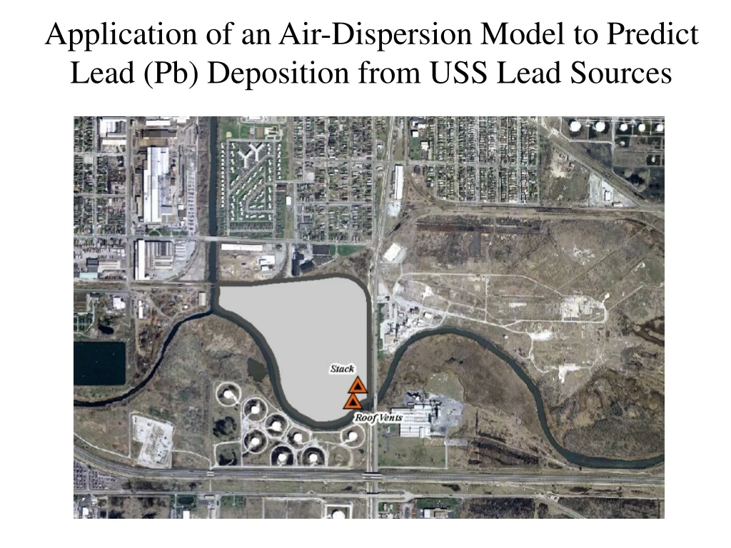
2. Application of an Air-Dispersion Model to Predict Lead (Pb) Deposition from USS Lead Sources BACKGROUND (from LAW, 2000): USS Lead operated on a 79-acre parcel of property in East Chicago, Indiana between the years 1920 and 1985. From 1920 to 1973, USS Lead operated a primary lead smelter on approximately 25 acres of the property. From 1973 to 1985, USS lead converted to secondary smelting operations. Soil samples collected from the early 1980s indicate elevated lead concentrations in properties near USS Lead. The lead smelting operations conducted at USS Lead may have contributed to lead contamination in the soils of residential and industrial properties surrounding the USS Lead facilities. In 1982, the Indiana Department of Environmental Management (IDEM) identified two fugitive sources of lead on USS Lead property, as well as other off-site sources. The two on-site sources include a single stack (point source) and roof vents (volume source). As part of a lead State Implementation Plan (SIP), IDEM documented the following source parameters: source heights, temperatures, diameters, exhaust gas velocities, and emission rates (Table 1). LAW. 2000. Independent Assessment of the Impacts of Historical Lead Air Emissions, USS Lead, East Chicago, Indiana. In Geochemical Solutions. Final USS Lead RCRA Facility Investigation (MRFI) Report. Submitted March 2004.

3. Application of an Air-Dispersion Model to Predict Lead (Pb) Deposition from USS Lead Sources • Table 1. Results of the SIP investigation that identified lead emission parameters for USS Lead. These parameters were used as inputs into the ISCST model. • * δyo = building width / 4.3 • ** δzo = building height / 2.15 AIR DISPERSION MODELING LAW (2000) conducted air dispersion modeling to evaluate the potential effects of lead emissions from USS Lead and other nearby industries on soils in the surrounding area. During this process, LAW used source parameters collected from the 1980’s by IDEM while developing the SIP. The Industrial Source Complex Short-Term (ISCST) model was used. ISC3 is a Gaussian plume, steady-state model capable of estimating close-distance impacts from industrial sources (EPA, 1995). This model can accommodate simple point source emission rates from stacks, as well as emission rates from piles, vents, and conveyor belts. Input parameters include meteorological data (wind speed, direction, etc.) as well as input parameters of the contaminant. This model was set up to output the average deposition rate in terms of grams per square meter per second (g/m2/second). In July 2006, the US EPA Region V FIELDS Team applied ISCST to model the deposition of lead emitted from USS Lead sources only. The FIELDS’ approach is different than that taken by LAW (2000) in that only fugitive emissions from USS Lead were used in the model, the FIELDS’ analysis used the effects of wet and dry depletion on lead deposition (whereas LAW [2000] neglected the effects of depletion), and the model output was set to calculate the average deposition rate in terms of grams per square meter per year (g/m2/year). The number of sources and their parameters used in the FIELDS’ analysis are identical to those used in LAW (2000). EPA. 1995. User’s Guide for the Industrial Source Complex (ISC3) Dispersion Models. Volume I: User Instructions. EPA-454/B-95-003a.

4. Application of an Air-Dispersion Model to Predict Lead (Pb) Deposition from USS Lead Sources AIR DISPERSION MODELING (cont’d) Yearly surface and precipitation meteorological data was obtained from the WebMET Meteorological Resource Center web site (www.webmet.com). A plotting program (WRPLOT View, Lakes-Environmental) was used to create a Wind Rose plot of the surface data. This Wind Rose plot shows the predominant wind pattern and is shown in Figure 1. The nearest weather station for this data was located in South Bend, Indiana (station # 14848) and was downloaded in SAMSON format for a 5-year period from 1986-1990. Upper air mixing height data was obtained from EPA’s Support Center for Regulatory Air Models (SCRAM) web site (http://epa.gov/ttn/scram/) using the nearest reported weather station (Peoria, IL, station # 14842). The meteorological data were compiled using the program PCRAMMET using the wet deposition option. The following local parameters were used in the PCRAMMET process:

5. FIGURE 1. Wind Rose plot of meteorological data collected for South Bend, Indiana, averaged for the years between 1986-1990. This Wind Rose diagram shows the direction to which the wind is blowing, which indicates a predominant from-southwest-to-northeast pattern. The resultant flow vector is 59 degrees.

6. Application of an Air-Dispersion Model to Predict Lead (Pb) Deposition from USS Lead Sources AIR DISPERSION MODELING (cont’d) A receptor grid of 468 radial samples was determined at a 10-degree flow vector in 200 m step-outs (maximum 2600 m) around the midpoint between the stack and volume sources at USS Lead. The terrain surrounding USS Lead is relatively flat; therefore, the model included rural control options without elevated receptors (see Fig. 2). Specific characteristics of the emitted lead molecules are identical to those reported by LAW (i.e., density & diameter). The model was run using the compiled meteorological data for the 5-year period and the lead deposition output was calculated as a 1-year average. The model output was saved in a separate plot file, which provided the x,y UTM coordinates of each receptor along with the wet and dry deposition of lead. Data from the plot file were exported into ArcGIS 9.1, where the data were viewed spatially. Inverse-Distance Weighted (IDW) interpolations were performed on annual wet and dry deposition estimates. Only interpolations of dry deposition estimates are shown in this report. For each concentric 200m radius extending out from the USS Lead receptor grid center, the deposition estimates were rank transformed and interpolated to show areas of highest lead deposition (regardless of deposition rate).

7. Application of an Air-Dispersion Model to Predict Lead (Pb) Deposition from USS Lead Sources FIGURE 2. The run-stream input file used in the ISCST model.

8. Application of an Air-Dispersion Model to Predict Lead (Pb) Deposition from USS Lead Sources MODELING RESULTS A summary of the output from the ISCST model is shown in Table 2. The interpolated dry depletion estimates were converted to contours and shown in Figure 3. The predominant dispersion pattern appears to be to the northeast and some dispersion to the southeast. Dry depletion results in considerably more deposition than wet depletion because it assumes no downwash from precipitation. This has been considered an appropriate assumption for modeling lead dispersion because lead is generally insoluble in water and the infrequency of rain events (LAW, 2000). Based upon this assumption, the annual deposition of lead from the USS Lead sources exceeds 2.5 g/m2 over an area of 9,372,826 m2 surrounding the USS Lead facility (as shown in blue on Fig. 3). Figure 4 shows the results of the interpolated rank-transformed dry deposition estimates. This figure clearly shows that predominant deposition pattern is to the northeast of the USS Lead facility. This corroborates with the Wind Rose diagram. TABLE 2. Summary of the ISCST model output for lead deposition around USS Lead.

9. FIGURE 3.

10. FIGURE 4.