Download
1 / 44
440 likes | 460 Views
This article explores the concepts of sound sampling, quantization, and psychoacoustics. It explains how sound waves are digitized and the effects of quantization on signal quality. It also discusses the frequency range of human hearing and the phenomenon of frequency masking and temporal masking.

E N D
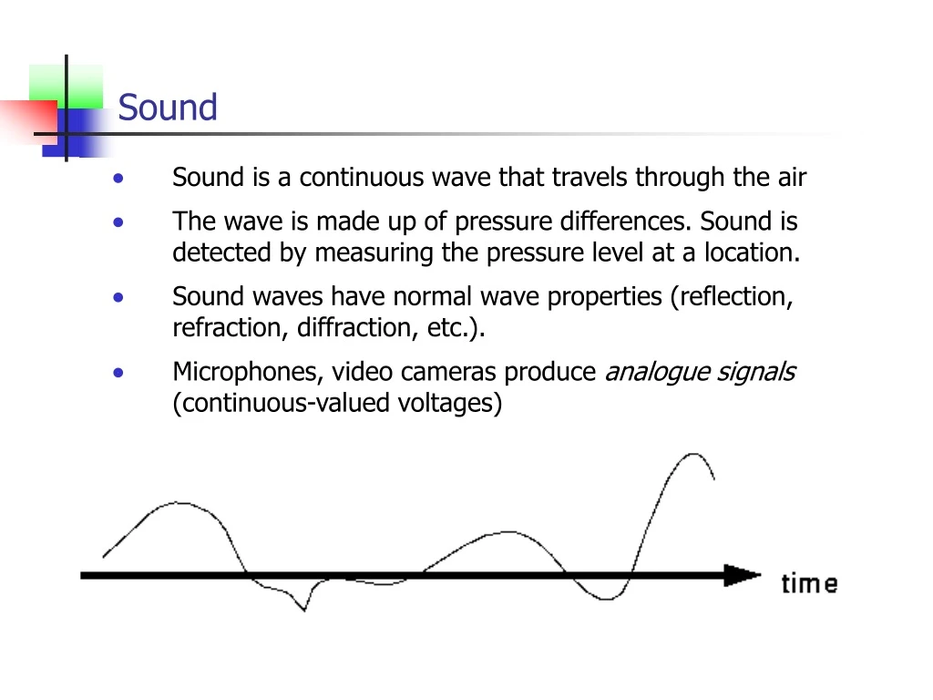
Sound • Sound is a continuous wave that travels through the air • The wave is made up of pressure differences. Sound is detected by measuring the pressure level at a location. • Sound waves have normal wave properties (reflection, refraction, diffraction, etc.). • Microphones, video cameras produce analogue signals (continuous-valued voltages)
SoundSampling and Quantisation • To get audio or video into a computer the analogue is digitized (converted into a stream of bits). The time and voltage axes are discreted by sampling and quantisation. • Sampling -- divide the horizontal axis (the time dimension) into discrete pieces. • Quantization -- divide the vertical axis (signal strength) into pieces. Sometimes, a non-linear function is applied. • 8 bit quantization divides the vertical axis into 256 levels. 16 bit gives you 65536 levels.
SoundNyquist Theorem • Given a Sine wave • Sample at 1 time per cycle and the result is a constant output • Sample at 1.5 times per cycle, and a lower frequency sine wave is obtained --> Alias • Nyquist rate -- For good digitization, the sampling rate should be at least twice of the maximum frequency.
SoundSignal to Noise Ratio (SNR) • In any analog system, some of the voltage is what you want to measure (signal), and some of it is random fluctuations (noise). • Ratio of the power of the two is called the signal to noise ratio (SNR). SNR is a measure of the quality of the signal • SNR is usually measured in decibels (dB).
SoundSignal to Quantization Noise Ratio (SQNR) • The precision of the digital audio sample is determined by the number of bits per sample, typically 8 or 16 bits. The quality of the quantization can be measured by the Signal to Quantization Noise Ratio (SQNR). • The quantization error (or quantization noise) is the difference between the actual value of the analog signal at the sampling time and the nearest quantization interval value. The largest (worst) quantization error is half of the interval. • Given N to be the number of bits per sample, the range of the digital signal is -2(N-1) to 2(N-1)-1. • In other words, each bit adds about 6 dB of resolution, so 16 bits enable a maximum SQNR = 96 dB.
SoundA-Law Non-Linear Quantisation • The A-law compander has a midriser and is defined by • for • for y Logarithmic part Linear part x
Soundm-Law Non-Linear Quantisation • The µ-law compander has a midtread and is defined by y Logarithmic part shifted to intersect at origin of axes x
Audio Formats • Popular audio file formats: • .au (Unix workstations), • .aiff (MAC, SGI), • .wav (PC, DEC workstations)
PsychoacousticsHuman hearing and voice • Human Hearing frequency range is about 20 Hz to 20 kHz, most sensitive at 2 to 4 KHz. • Dynamic range (quietest to loudest) is about 96 dB • Normal voice range is about 500 Hz to 2 kHz • Low frequencies are vowels and bass • High frequencies are consonants
Psychoacoustics Sensitivity of human hearing against frequency • Experiment: Put a person in a quiet room. Raise level of 1 kHz tone until just barely audible. Vary the frequency and plot • Graph shows hearing is more sensitive to low frequencies
Psychoacoustics Frequency Masking • Experiment: Play 1 kHz tone (maskingtone) at fixed level (60 dB). Play test tone at a different level (e.g., 1.1 kHz), and raise level until just distinguishable. Vary the frequency of the test tone and plot the threshold when it becomes audible: • Repeat for various frequencies of masking tones
PsychoacousticsCritical Bands • Human auditory system has a limited, frequency-dependent resolution. The perceptually uniform measure of frequency can be expressed in terms of the width of the Critical Bands.It is less than 100 Hz at the lowest audible frequencies, and more than 4 kHz at the high end. Altogether, the audio frequency range can be partitioned into 25 critical bands. • A new unit for frequency bark (after Barkhausen): • 1 Bark = width of one critical band • Dynamic range (quietest to loudest) is about 96 dB • Normal voice range is about 500 Hz to 2 kHz • Low frequencies are vowels and bass • High frequencies are consonants • For frequency < 500 Hz, it converts to freq / 100 Bark, • For frequency > 500 Hz, it is Bark.
Psychoacoustics Temporal masking • If we hear a loud sound, then it stops, it takes a little while until we can hear a soft tone nearby. • Experiment: Play 1 kHz masking tone at 60 dB, plus a test tone at 1.1 kHz at 40 dB. Test tone can't be heard (it's masked). • Stop masking tone, then stop test tone after a short delay. • Adjust delay time to the shortest time when test tone can be heard (e.g., 5 ms). • Repeat with different level of the test tone and plot:
PsychoacousticsEffect of both frequency and temporal maskings
Audio CompressionPulse Code Modulation • A Continuous time analogue signal is put through a low pass anti-alias filter before being sampled to generate a Pulse Amplitude Modulated (PAM) signal. • PCM is a technique which quantises the PAM signal into N levels and encodes each quantised sample into a digital word of b bits (b = log2(N)). • The receiver only distinguishes between digital levels 0 and 1. This has a degree of immunity to interference and noise on a channel that is obtained at the cost of a small error in the message representation (error due to quantisation). • The sampled analogue signal is low pass filtered to recover the reconstructed analogue signal.
Audio CompressionDifferential PCM • The prediction error of the nth sample d(n) is the difference between the next measured sample X(n) and the predicted sample Xp(n). • The transmitter forms a prediction correction Xc(n) by performing the sum of its prediction Xp(n) and the prediction error d(n).
Audio CompressionDifferential PCM dn is sent and then used to correct the Xp(n) to get Xc(n)=X(n) Xp(n) d(n) X(n) = Xc(n) = Xp(n) + d(n)
Audio Compression: Differential PCMNumber of Taps on Prediction filter • A N-tap linear prediction coding (LPC) filter predicts the next sample based on a linear combination of the previous N samples values. • A predictor order which is greater than 10 does not significantly improve the input signal to prediction error power ratio.
Audio CompressionAdaptive DPCM • Adaptive encoders incorporate (long time) auxiliary loops to estimate the parameters required to obtain time local optimal performance. • These auxiliary loops periodically schedule modifications to the prediction loop parameters and thus avoid predictor mismatch. • The update rate of the adaptive coefficients is related to the length of the time the input signal can be considered locally stationary e.g speech is caused by mechanical displacement of the speech articulators (tongue, lips, teeth etc) which can not change more rapidly than 10 or 20 times per second suggesting an interval of 50-100ms.
Audio CompressionDigital Circuit Multiplication Equipment (DCME) • Equipment using a combination of ADPCM low rate encoding techniques and Digital Speech interpolation is referred to as Digital Circuit Multiplication Equipment (DCME). • The DCME equipment uses the silent parts of the speech to insert someone else's speech. and steals bits from speech channels to create new speech channels.
Audio CompressionDCME - Silent period suppression • Analyses of telephone conversations have indicated that a source is typically active about 40% of a call duration. Most inactivity occurs as a result of one person listening while the other is talking. Thus a full duplex connection (simultaneous communication in both directions) is significantly under utilised. • Digital Speech Interpolation (DSI) sense speech activity, seizes a channel, digitally encodes information, transmits it and releases the channel at the completion of each speech segment. DSI is only applicable when the duration of the pause can be encoded more efficiently than the pause itself.
Audio CompressionDCME - Silent period suppression • ADPCM provides good quality speech at 32kbit/s (4bits/channel on a 30 channel frame at 125s per frame) and may be marginally acceptable at 24kbit/s (3bits/channel on a 40 channel frame at 125s per frame) although it is noticeably inferior to 64kbit/s PCM and at 16kbit/s (2bits/channel on a 60 channel frame at 125s per frame) . • When the traffic becomes very busy a bit is stolen from the ADPCM speech at 4bits per channel, for a short period of time so that there is an average of less than 4 bits per channel. The increase in quantisation distortion is not heard because the bits are only stolen for a few msec at a time. • A speech/data discriminator identifies whether the activity detected by the activity detector is speech data or signalling. It does this by examining the energy level, peak to mean ratio of the signal envelope and the signal power spectrum. On an analogue telephone line, the peak to mean ratio remains constant for data whereas it varies for speech and the signal power spectrum is restricted to a number of individual tones for signalling where as is the whole bandwidth is used in speech.
Audio CompressionCode Excited Linear Prediction • When the filter coefficients of a 10-tap predictive coder are periodically computed with an optimal algorithm every 30ms or 240 samles, the prediction removes short term correlations in the sampled speech. • A long term predictor (or pitch predictor) is used to model the fine structure of the long term spectral envelope of speech. The short term prediction error exhibits periodicity which is related to the pitch period of the original speech. This periodicity is of the order of 20-160 sample intervals. The long term predictor removes the pitch periodicity. The long term predictor is usually a 1 tap predictor whose lag is optimally determined over 20 160. • After the long and short term predictor have removed the periodic signals from the speech, the resultant signal is excitation noise.
Audio CompressionCode Excited Linear Prediction • The filter A(z)-1 computes the long term and short term predictions of the speech structure. • The theory of auditory masking suggests that the excitation noise in the formant regions are partially or totally masked by the speech signal. • A large part of the excitation noise in a coder comes from the frequency regions where the signal level is low. Therefore to reduce the excitation noise its flat spectrum is shaped so that the frequency components of the noise around the formant regions are allowed to have a higher energy relative to the components in the inter-formant regions. The parameters of the shaping filter A(Z/g) are chosen to weight the frequency components of the excitation noise to reduce it in the inter-formant regions of the spectrum.
Audio CompressionMELP, CELP, VSELP, ACELP • There are many ways in which the excitation signal can be generated: • Multi-pulse Excited Linear Predictor (MELP): allows several (multiple) impulses to be used as the synthesis filter excitation over a frame of speech. The pulse amplitudes and positions are determined one at a time for minimising the mean squared error between the original and synthesised speech. • Codebook Excited Linear Predictor (CELP): the prediction errors in a 30ms interval are compared (cross correlated) with a codebook of prediction errors and the code for the best match is transmitted and used as the excitation input at the receiver. Offline training is used to produce the codebooks. • Algebraic CELP (ACELP) restricts the codebook to have pulse amplitudes that all have the same amplitude level. The quality of the synthesised speech is not effected and the search for the code is greatly simplified. • Vector Sum Excited Linear Predictor (VSELP): This is the same as the CELP except that it uses two codebooks (as opposed to one) to increase the variety of codes that can be generated whilst keeping complexity down.
Audio CompressionSub-band Codec • The speech spectrum is filtered into sub-bands using band pass filtered centered around different frequencies (fn where n=1..5) in the frequency domain. Each sub-band is coded using a sampling rate equal to twice the bandwidth in each case. • If the bands are made as narrow as the ear's critical bands the quantising noise is largely masked by the speech signal within the same band e.g. the ear can not resolve tones within the bands. For 'unvoiced' randomly excited sounds, the waveform shape in the higher bands need not be specified so accurately and therefore require fewer bits. At the receiver the sampled and encoded waveforms are decoded and recovered using corresponding band pass filters.
MPEG-1 Audio Compression • MPEG-1: 1.5 Mbits/sec for audio and video • About 1.2 Mbits/sec for video, 0.3 Mbits/sec for audio • Compression factor ranging from 2.7 to 24. • With Compression rate 6:1 (16 bits stereo sampled at 48 KHz is reduced to 256 kbits/sec) and optimal listening conditions, expert listeners could not distinguish between coded and original audio clips. • MPEG audio supports sampling frequencies of 32, 44.1 and 48 KHz. • Supports one or two audio channels in one of the four modes: • Monophonic -- single audio channel • Dual-monophonic -- two independent channels, e.g., English and French • Stereo -- for stereo channels that share bits, but not using Joint-stereo coding • Joint-stereo -- takes advantage of the correlations between stereo channels
MPEG-1 Audio Compression: Algorithm • Use convolution filters to divide the audio signal (e.g., 48 kHz sound) into 32 frequency subbands --> subband filtering. • Determine amount of masking for each band caused by nearby band using the psychoacoustic model shown above. • If the power in a band is below the masking threshold, don't encode it. • Otherwise, determine number of bits needed to represent the coefficient such that noise introduced by quantization is below the masking effect (Recall that one fewer bit of quantization introduces about 6 dB of noise). • Format bitstream
MPEG-1 Audio Compression: Example • After analysis, the first levels of 16 of the 32 bands are these: • If the level of the 8th band is 60dB, it gives a masking of 12 dB in the 7th band, 15dB in the 9th. • Level in 7th band is 10 dB ( < 12 dB ), so ignore it. • Level in 9th band is 35 dB ( > 15 dB ), so send it. [ Only the amount above the masking level needs to be sent, so instead of using 6 bits to encode it, we can use 4 bits -- a saving of 2 bits (= 12 dB). ]
MPEG Audio Compression: Grouping of Subband Samples for Layer 1, 2, and 3 • MPEG defines 3 layers for audio. Basic model is same, but codec complexity increases with each layer. • Divides data into frames, each of them contains 384 samples, 12 samples from each of the 32 filtered subbands as shown below.
MPEG Audio Compression: Grouping of Subband Samples for Layer 1, 2, and 3 • A perceptual subband audio encoder constantly analyses the incoming audio signal and determines the so-called masking curve, the threshold under which additional noise will not be audible by the human auditory system. • Divides data into frames, each of them contains 384 samples, 12 samples from each of the 32 filtered subbands as shown below.
MPEG-1 Audio Compression: Layer 1, 2, and 3 • Layer 1: DCT type filter with one frame and equal frequency spread per band. Psychoacoustic model only uses frequency masking. • Layer 2: Use three frames in filter (before, current, next, a total of 3*384=1152 samples). This models a little bit of the temporal masking. • Layer 3: Better critical band filter is used (non-equal frequencies), psychoacoustic model includes temporal masking effects, takes into account stereo redundancy, and uses Huffman coder. • Intensity stereo coding -- at upper-frequency subbands, encode summed signals instead of independent signals from left and right channels. • Middle/Side (MS) stereo coding -- encode middle (sum of left and right) and side (difference of left and right) channels.
MPEG-2 Audio CompressionSurround Sound audio coding • MPEG-2 creates a multichannel movie theatre sound system and hence caters for surround sound channels. • The audio output for the L speaker can be derived from the audio output of the L, C and Ls speakers for downward compatibility, where L0= L + (C/2 ) + (LS/2 ) and R0= R + (R/2 ) + (RS/2 ) • There can be various channel designations
MPEG-2 Audio CompressionMPEG-2 Forward Compatibility with MPEG-1 • For forward compatible audio, MPEG-2 can decode MPEG-1 bit stream. • For forward compatibility it is the responsibility of MPEG-2 decoder to deal with the MPEG-1 bit stream to drive its left and right channel speakers.
MPEG-2 Audio CompressionMPEG-2 Backward Compatibility with MPEG-1 • For backward compatible audio, MPEG-1 can decode MPEG-2 multichannel bit stream. • Downward compatibility with MPEG-1 is achieved by using downward mixing equations L0= L + (n x C) + (m x LS) R0= R + (n x C) + (m x RS) where possible values of n = m = 1/21/2
MPEG-2 Audio CompressionMPEG-2 Backward Compatibility with MPEG-1 • MPEG-1 decoder is able to decode properly an MPEG-2 audio bit stream by inserting the MPEG-2 extension signal in the MPEG-1 auxiliary data field.
MPEG-2 Audio CompressionMPEG-2 Backward Compatibility with MPEG-1 • L0 and R0 are transmitted on channels T0 and T1 and encoded by MPEG-1 encoder. • C, LS and RS are transmitted on channels T2 , T3 and T4 and encoded by MPEG-2 encoder. • MPEG-2 Layers 1,2,3 are similar to those of MPEG-1 except that it is capable of using lower sampling frequencies.