Threshold Autoregressive
Threshold Autoregressive. Several tests have been proposed for assessing the need for nonlinear modeling in time series analysis Some of these tests, such as those studied by Keenan (1985 )

Threshold Autoregressive
E N D
Presentation Transcript
Several tests have been proposed for assessing the need for nonlinear modeling in time series analysis • Some of these tests, such as those studied by Keenan (1985) • Keenan’s test is motivated by approximating a nonlinear stationary time series by a second-order Volterra expansion (Wiener,1958)
where {εt, −∞ < t < ∞} is a sequence of independent and identically distributed zero-mean random variables. • The process {Yt} is linear if the double sum on the righthandside vanishes
where the φ’s are autoregressive parameters, σ’s are noise standard deviations, r is the threshold parameter, and {et} is a sequence of independent and identically distributed random variables with zero mean and unit variance
The process switches between two linear mechanisms dependent on the position of the lag 1 value of the process. • When the lag 1 value does not exceed the threshold, we say that the process is in the lower (first) regime, and otherwise it is in the upper regime. • Note that the error variance need not be identical for the two regimes, so that the TAR model can account for some conditional heteroscedasticityin the data.
As a concrete example, we simulate some data from the following first-order TAR model:
Exhibit 15.8 shows the time series plot of the simulated data of size n = 100 Somewhat cyclical, with asymmetrical cycles where the series tends to drop rather sharply but rises relatively slowly time irreversibility (suggesting that the underlying process is nonlinear)
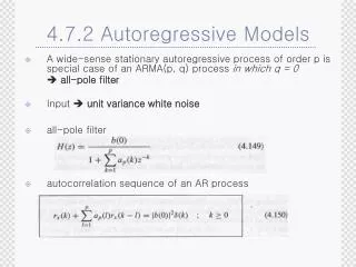
Threshold Models • The first-order (self-exciting) threshold autoregressive model can be readily extended to higher order and with a general integer delay: 15.5.1 Note that the autoregressive orders p1 and p2 of the two submodels need not be identical, and the delay parameter d may be larger than the maximum autoregressive orders
However, by including zero coefficients if necessary, we may and shall henceforth assume that p1 = p2 = p and 1 ≤ d ≤ p, which simplifies the notation. • The TAR model defined by Equation (15.5.1) is denoted as the TAR(2;p1, p2) model with delay d. • TAR model is ergodic and hence asymptotically stationary if |φ1,1|+…+ |φ1,p| < 1 and |φ2,1| +…+ |φ2,p| < 1
The extension to the case of m regimes is straightforward and effected by partitioning the real line into −∞ < r1 < r2 <…< rm − 1 < ∞, and the position of Yt − d relative to these thresholds determines which linear submodel is operational
While Keenan’s test and Tsay’s test for nonlinearity are designed for detecting quadratic nonlinearity, they may not be sensitive to threshold nonlinearity • Here, we discuss a likelihood ratio test with the threshold model as the specific alternative • The null hypothesis is an AR(p) model • the alternative hypothesis of a two-regime TAR model of order p and with constant noise variance, that is; σ1 = σ2 = σ
The general model can be rewritten as where the notation I(⋅) is an indicator variable that equals 1 if and only if the enclosed expression is true In this formulation, the coefficient φ2,0 represents the change in the intercept in the upper regime relative to that of the lower regime, and similarly interpreted are φ2,1,…,φ2,p
The null hypothesis states that φ2,0 = φ2,1 =…= φ2,p= 0. • While the delay may be theoretically larger than the autoregressive order, this is seldom the case in practice. • Hence, it is assumed that d ≤ p
The test is carried out with fixed p and d. • The likelihood ratio test statistic can be shown to be equivalent to where n − p is the effective sample size, is the maximum likelihood estimator of the noise variance from the linear AR(p) fit and from the TAR fit with the threshold searched over some finite interval
Hence, the sampling distribution of the likelihood ratio test under H0 is no longer approximately χ2 with p degrees of freedom. • Instead, it has a nonstandard sampling distribution; see Chan (1991) and Tong (1990) • Chan (1991) derived an approximation method for computing the p-values of the test that is highly accurate for small p-values. • The test depends on the interval over which the threshold parameter is searched. • Typically, the interval is defined to be from the a×100th percentile to the b×100th percentile of {Yt}, say from the 25th percentile to the 75th percentile • The choice of a and b must ensure that there are adequate data falling into each of the two regimes for fitting the linear submodels.
Estimation of a TAR Model • If r is known, the estimation of a TAR model is straightforward. • Separate the observation according to whether Yt-1 is above or below the threshold • Each segment of TAR model can then be estimated using OLS. • The lag lenghts p1 and p2 can be determined as in AR model
A simple numerical example might be helpful. • Suppose that the first seven observations of a time series are as follow : • If you know that threshold is zero, sort the observation into two groups according to whether Yt-1 is greater that or less than zero
The two regime would look like this; • The two separate AR(p) processes can be estimated for each regime
If we restrict var (1t) = var (2t), we can rewrite TAR model as (*) • Where It=1 if Yt-1> r and It = 0 if Yt-1 ≤ 0 • So that if Yt-1> r, It=1 and 1 - It= 0
if Yt-1 ≤ 0, It=0 and 1 - It= 1 • To estimate a TAR model in the form (*), create the indicator function and form the variables ItYt-i and (1 – It)Yt-i. • You can then estimate the equation using OLS
To estimate the model using one lag in each regime, you estimate the model using the 4 variabel. • To estimate the model using two lag in each regime, you estimate the model using the 6 variabel
Unknown Threshold (r) • r must lie between the maximum and minimum value of the series • Try a value of r = y1( the first observation in the band) and estimate an equation • If y2 lies outside the band, there is no need to estimate TAR model using r = y2 • Next estimate TAR model using r = y3. • Continue in this fashion for each observation within the band • The regression containing the smallest residual sum of squares contains the consistent estimate of the threshold.
Selecting the Delay Parameter • The standar procedure is to estimate a TAR model for each potential value of d • The model with the smallest value of the residual sum of squares contains the most appropriate value of the delay parameter. • Alternatively, choose the delay parameter that leads to the smallest value of the AIC or the SBC
Model Diagnostics Model diagnostics via residual analysis • The time series plot of the standardized residuals should look random, as they should be approximately independent and identically distributed if the TAR model is the true data mechanism; that is, if the TAR model is correctly specified
The independence assumption of the standardized errors can be checked by examining the sample ACF of the standardized residuals. • Nonconstant variance may be checked by examining the sample ACF of the squared standardized residuals or that of the absolute standardized residuals