Introduction to Operations Research and Linear Programming
960 likes | 1.79k Views
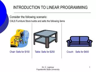
Introduction to Operations Research and Linear Programming. Kanjana Thongsanit Silpakorn University. Introduction. Our world is filled with limited resources. Oil Land Human Time Business Resource (Budget) Manufacturing m/c , number of worker Restaurant

Introduction to Operations Research and Linear Programming
E N D
Presentation Transcript
Introduction to Operations Research and Linear Programming KanjanaThongsanit Silpakorn University
Introduction • Our world is filled with limited resources. • Oil • Land • Human • Time • Business • Resource (Budget) • Manufacturing • m/c , number of worker • Restaurant • Space available for seating
Introduction • How best to used the limited resources available ? • How to allocate the resource in such a way as to maximize profits or minimize costs ?
Introduction • Mathematical Programming(MP) is a field of management science or operations research that fines most efficient way of using limited resources/ to achieve the objectives of a business. Optimization
Characteristics of Optimization Problems • One or more decisions • Restrictions or constraints e.g. Determining the number of products to manufacture a limited amount of raw materials a limited amount of labor • Objective • The production manager will choose the mix of products that maximizes profits • Minimizing the total transportation cost
Expressing optimization problems mathematically • Decision variables X1 , X2 , X3 , … , Xn e.g. the quantities of different products Index n = the number of product types • Constraints • a less than or equal to constraint : f(X1 , X2 , X3 , … , Xn) < b • a greater than or equal to constraint : f(X1 , X2 , X3 , … , Xn) > b • an equal to constraint : f(X1 , X2 , X3 , … , Xn) = b • Objective • MAX(or MIN) : f(X1 , X2 , X3 , … , Xn)
Mathematical formulation of an optimization problem MAX(or MIN) : f(X1 , X2 , X3 , … , Xn) Subject to: f(X1 , X2 , X3 , … , Xn) < b1 …. f(X1 , X2 , X3 , … , Xn) >bk …. f(X1 , X2 , X3 , … , Xn) = bm note : n variables , m constraints
Mathematical programming techniques Test : Linear functions? 1. 2. 3. 4. 5.
Problem • Blue Ridge Hot Tubs manufactures and sells two models of hot tubs : Aqua Spa and the Hydro-Lux. • Howie Jones, the owner and manager of the company, needs to decide how many of each type of hot tubs to produce • 200 pumps available • Howie expects to have 1,566 production labor hours and 2,880 feet of tubing available. • Aqua-Spa requires 9 hours of labor and 12 feet of tubing • Hydro-Lux require s 6 hours of labor and 16 feet of tubing Assuming that all hot tubs can be sold To maximize profits, how many Aqua-Spas and Hydra-Luxs should be produce?
Formulating LP Models 1. Understand the problem 2. Indentify the decision variable 3. State the objective as a linear combination of decision variables Max : 350x1 + 300x2 4. State the constraints as linear combinations of the decision variable 4.1 Pumps available 4.2 labor available 4.3 Tubing available 5. Identify any upper or lower bounds on the decision variable x1> 0 x2> 0
Max : 350x1 + 300x2 Subject to: x1 +x2 < 200 , Pumps available 9x1 + 6x2 < 1,566 , Labors available 12x1 + 16x2 < 2,880 , Tubing available x1 > 0 x2 > 0
General Form of an LP model MAX(or MIN) : C1X1+ C2X2+ , … , CnXn Subject to: a11X1+ a12X2+ , … , a1nXn< b1 ak1X1+ ak2X2+ , … , aknXn> bk am1X1+ am2X2+ , … , amnXn = bm
Notations a11X1+ a12X2+ , … , a1nXn< b1 X1+ X2+, … ,+ Xn = b1 X11 + X21+ X31 = b1 X12 + X22+ X32 = b2
Graphical Method: Solving LP Problems
Graphical Method x1+x2 ≤ 200 (1)
Graphical Method x1+x2 ≤ 200 (1) 9x1+ 6x2 ≤ 1,566 (2) Note : X1 = 0 , x2 = 1566/6 = 261 X2 = 0 , x1 = 1566/9 =174
Graphical Method x1+x2 ≤ 200 (1) 9x1+ 6x2 ≤ 1,566 (2) 12x1+ 16x2 ≤ 2,880 (3) Note : X1 = 0 , x2 = 2880/16 = 180 X2 = 0 , x1 = 2880/12 = 240
Graphical Method MAX 350x1 + 300x2
Using level curves • MAX 350x1 + 300x2 1. Set a number of objective e.g. Obj = 35,000 2. Finding points (x1,x2) which has obj = 35,000 x1 = 100 , x2 = 0 x1 = 0 , x2 = 116.67
Graphical Method MAX 350x1 + 300x2 x1+x2 ≤ 200 (1) 9x1+ 6x2 ≤ 1,566 (2) 12x1+ 16x2 ≤ 2,880 (3)
Finding the optimal solution x1+x2 = 200 (1) 9x1+ 6x2 = 1,566 (2) 9x1+ 6(200 –x1) = 1,566 3x1+ 1,200 = 1,566 3x1 = 366 Optimal Solution = x1 = 122 X2 = 78
Special Conditions in LP Models • Alternate Optimal Solutions • - having more than one optimal solution MAX 450x1 + 300x2 x1+x2 ≤ 200 (1) 9x1+ 6x2 ≤ 1,566 (2) 12x1+ 16x2 ≤ 2,880 (3)
Special Conditions in LP Models 2. Redundant Constraints A constraint that plays no role in determining the feasible region of the problem. MAX 350x1 + 300x2 x1+x2 ≤ 225 (1) 9x1+ 6x2 ≤ 1,566 (2) 12x1+ 16x2 ≤ 2,880 (3)
Special Conditions in LP Models 3. Unbounded Solutions The objective function can be made infinitely large. MAX x1 + x2 x1+ x2 ≥ 400 (1) -x1+ 2x2 ≤ 400 (2) x1 ≥ 0 x2 ≥ 0
Special Conditions in LP Models 4. Infeasibility • No ways to satisfy all of the constraints ? MAX x1 + x2 x1+ x2 ≤ 150 (1) x1+ x2 ≥ 200 (2) x1 ≥ 0 x2 ≥ 0
Using Excel Solver MAX 350x1 + 300x2 x1+x2 ≤ 200 (1) 9x1+ 6x2 ≤ 1,566 (2) 12x1+ 16x2 ≤ 2,880 (3)
Modeling LP Problems • Make vs. Buy Decisions - The Electro-Poly corporation received a $750,000 order for various quantities of 3 types of slip rings. - Each slip ring requires a certain amount of time to wire and hardness. The company has only 10,000 hours of wiring capacity. The company has only 5,000 hours of harnessing capacity.
Make vs. Buy Decisions (Continue) The company can sub contract to one of its competitors. Determine the number of slip rings to make and the number to buy in order to fill the customer order at the least possible cost
Make vs. Buy Decisions (Continue) • Defining the decision variables mi = number of model islip rings to make in-house bi = number of model islip rings to buy from competitor • Defining the objective function • To minimize the total cost Min : 50m1 + 83m2 + 130m3 + 61b1+ 97b2 + 145b3 Subject to: 2m1 +1.5m2 + 3m3< 10,000 , wiring constraint 1m1 +2m2 + m3< 5,000 , harness constraint m1 + b1 = 3,000 , Required order of model1 m2 + b2 = 2,000 , Required order of model2 m3 + b3 = 900 , Required order of model3 m1 ,m2 ,m3 , b1 ,b2 ,b3 , > 0
A transportation problem Supply R/M Area Processing Plant Capacity 275,000 200,000 400,000 600,000 300,000 225,000 i1 j1 i2 j2 i3 j3
A transportation problem • How many product should be shipped from r/m area to the processing plant, the trucking company charges a flat rate for every mile. Min the total distance ~ Min total cost of transportation • Defining the decision variable xij= number of R/M to ship from node i to node j • Defining the objective function Min : 21x11+50x12 +40x13+35x21 +30x22 +22x23 +55x31 +20x32 +25x33 • Defining the constraints x11 +x21 + x31< 200,000 capacity restriction for j1 x12 +x22 + x32< 600,000 capacity restriction for j2 x13 +x23 + x33< 225,000 capacity restriction for j3 x11 +x12 + x13 = 275,000 supply restriction for i1 x21 +x22 + x23 = 400,000 supply restriction for i2 x31 +x32 + x33 = 300,000 supply restriction for i3 xij > 0 , for all i and j
A Blending problem • Agri-Pro stocks bulks amounts of four types of feeds that can mix to meet a given customer’s specifications.
A Blending problem • Agri-Pro has just received an order from a local chicken farmer for 8,000 pounds of feed. • The farmers wants this feed to contain at least 20% corn, 15% grain , and 15% minerals. • What should Agri-Pro do to fill this order at minimum cost? • Defining the decision variable xi = pounds of feed (j) to use in the mix • Defining the objective function Min : 0.25x1 +0.30x2 +0.35x3+0.15x4 , total cost • Defining the constraints x1 +x2 + x3 + x4 = 8,000 0.3x1 +0.05x2 + 0.20x3 + 0.10x4> 0.20 × 8,000 --- Corn 0.1x1 +0.30x2 + 0.15x3 + 0.10x4> 0.15× 8,000 --- Grain 0.2x1 +0.20x2 + 0.20x3 + 0.30x4> 0.15 × 8,000 --- Mineral x1 , x2 , x3 , x4 > 0
A production and inventory planning problem • Upton Corporation is trying to plan its production and inventory levels for the next 6 months • Given the size of Upton’s warehouse, a maximum of 6,000 units • The owner like to keep at least 1,500 units in inventory any months as safety stock • The company wants to produce at no less than half of its maximum production capacity each month. • Estimate that the cost of carrying a unit in any given month is equal to 1.5% of the unit production cost in the same month.
A production and inventory planning problem • The number of units carried in inventory using the averaging the beginning and ending inventory for each month • Current inventory 2,750 units • To minimize production and inventory costs, the company wants to identify the production and inventory plan. • Defining the decision variable pm = the number of units to product in month m bm = the beginning inventory for month m
A production and inventory planning problem • Defining the objective function Min : , Subject to