Download
1 / 57
570 likes | 794 Views
Markov Chains, Markov Decision Processes (MDP), Reinforcement Learning: A Quick Introduction. Hector Munoz-Avila Stephen Lee-Urban Megan Smith www.cse.lehigh.edu/~munoz/InSyTe. Disclaimer. Our objective in this lecture is to understand the MDP problem

E N D
Markov Chains, Markov Decision Processes (MDP), Reinforcement Learning: A Quick Introduction Hector Munoz-Avila Stephen Lee-Urban Megan Smith www.cse.lehigh.edu/~munoz/InSyTe
Disclaimer • Our objective in this lecture is to understand the MDP problem • We will touch on the solutions for the MDP problem • But exposure will be brief • For an in-depth study of this topic take CSE 337/437 (Reinforcement Learning)
Learning • Supervised Learning • Induction of decision trees • Case-based classification • Unsupervised Learning • Clustering algorithms • Decision-making learning • “Best” action to take (note about design project)
Applications • Fielded applications • Google’s page ranking • Space Shuttle Payload Processing Problem • … • Foundational • Chemistry • Physics • Information Theory
Some General Descriptions • Agent interacting with the environment • Agent can be in many states • Agent can take many actions • Agent gets rewards from the environment • Agents wants to maximize sum of future rewards • Environment can be stochastic • Examples: • NPC in a game • Cleaning robot in office space • Person planning a career move
Quick Example: Page Ranking • The “agent” is a user browsing pages and following links from page to page • We want to predict the probability P() that the user will visit each page • States: the N pages that the user can visit: A, B, C,… • Action: following a link • P() is a function of: • {P(’): ’ point to } • Special case: No rewards defined (Figure from Wikipedia)
Example with Rewards: Games • A number of fixed domination locations. • Ownership: the team of last player to step into location • Scoring: a team point awarded for every five seconds location remains controlled • Winning: first team to reach pre-determined score (50) (top-down view)
Rewards In all of the following assume a learning agent taking an action • What would be a reward in a game where agent competes versus an opponent? • Action: capture location B • What would be a reward for an agent that is trying to find routes between locations? • Action: choose route D • What is the reward for a person planning a career move • Action: change job
Objective of MDP • Maximize the future rewards • R1 + R2 + R3 + … • Problem with this objective?
Objective of MDP: Maximize the Returns • Maximize the sum R of future rewards • R = R1 + R2 + R3 + … • Problem with this objective? • R will diverge • Solution: use discount parameter (0,1) • Define: R = R1 + R2 + 2 R3 + … • R converges if rewards have upper bounds • R is called the return • Example: Monetary rewards and inflation
The MDP problem • Given: • States (S), actions (A), rewards (Ri), • A model of the environment: • Transition probabilities: Pa(s,s’) • Reward function: Ra(s,s’) • Obtain: • A policy *: S A [0,1] such that when * is followed, the returns R are maximized
Example • What will be the optimal policy for: (figures from Sutton and Barto book)
Requirement: Markov Property • Also thought of as the “memoryless” property • A stochastic process is said to have the Markov property if the probability of state Xn+1 having any given value depends only upon state Xn • In situations were the Markov property is not valid • Frequently, states can be modified to include additional information
Markov Property Example • Chess: • Current State: The current configuration of the board • Contains all information needed for transition to next state • Thus, each configuration can be said to have the Markov property
Obtain V(S)(V(s) = approximate “Expected return when reaching s”) • Let us derive V(s) as a function of V(s’)
Obtain (S)((s) = approximate “Best action in state s”) • Let us derive (s)
Policy Iteration (figures from Sutton and Barto book)
Solution to Maze Example (figures from Sutton and Barto book)
Reinforcement Learning Motivation: Like MDP’s but this time we don’t know the model. That is the following is unknown: Transition probabilities: Pa(s,s’) Reward function: Ra(s,s’) Examples?
Some Introductory RL Videos • http://www.youtube.com/watch?v=NR99Hf9Ke2c • http://www.youtube.com/watch?v=2iNrJx6IDEo&feature=related
UT Domination Games • A number of fixed domination locations. • Ownership: the team of last player to step into location • Scoring: a team point awarded for every five seconds location remains controlled • Winning: first team to reach pre-determined score (50) (top-down view)
Reinforcement Learning • Agents learn policies through rewards and punishments • Policy - Determines what action to take from a given state (or situation) • Agent’s goal is to maximize returns (example) • Tabular Techniques • We maintain a “Q-Table”: • Q-table: State × Action value
The DOM Game • Wall • Spawn Points • Domination Points Lets write on blackboard: a policy for this and a potential Q-table
Example of a Q-Table ACTIONS STATES “good” action Best action identified so far “bad” action For state “EFE” (Enemy controls 2 DOM points)
Reinforcement Learning Problem ACTIONS STATES How can we identify for every state which is the BEST action to take over the long run?
Let Us Model the Problem of Finding the best Build Order for a Zerg Rush as a Reinforcement Learning Problem
Adaptive Game AI with RL RETALIATE (Reinforced Tactic Learning in Agent-Team Environments)
The RETALIATE Team • Controls two or more UT bots • Commands bots to execute actions through the GameBots API • The UT server provides sensory (state and event) information about the UT world and controls all gameplay • Gamebots acts as middleware between the UT server and the Game AI
State Information and Actions Player Scores Team Scores Domination Loc. Ownership Map TimeLimit Score Limit Max # Teams Max Team Size Navigation (path nodes…) Reachability Items (id, type, location…) Events (hear, incoming…) SetWalk RunTo Stop Jump Strafe TurnTo Rotate Shoot ChangeWeapon StopShoot x, y, z
Managing (State x Action) Growth • Our Table: • States: ( {E,F,N}, {E,F,N}, {E,F,N} ) = 27 • Actions: ( {L1, L2, L3}, …) = 27 • 27 x 27 = 729 • Generally, 3#loc x #loc#bot • Adding health, discretized (high, med, low) • States: (…, {h,m,l}) = 27 x 3 = 81 • Actions: ( {L1, L2, L3, Health}, … ) = 43 = 64 • 81 x 64 = 5184 • Generally, 3(#loc+1) x (#loc+1)#bot • Number of Locations, size of team frequently varies.
Initialization • Game model: • n is the number of domination points • (Owner1, Owner2, …, Ownern) • For all states s and for all actions a • Q[s,a] 0.5 • Actions: • m is the number of bots in team • (goto1, goto2, …, gotom) • Team 1 • Team 2 • … • None • loc 1 • loc 2 • … • loc n
Rewards and Utilities • U(s) = F( s ) – E( s ), • F(s) is the number of friendly locations • E(s) is the number of enemy-controlled locations • R = U( s’ ) – U( s ) • Standard Q-learning ([Sutton & Barto, 1998]): • Q(s, a) ← Q(s, a) + ( R + γ maxa’Q(s’, a’) – Q(s, a))
Rewards and Utilities • U(s) = F( s ) – E( s ), • F(s) is the number of friendly locations • E(s) is the number of enemy-controlled locations • R = U( s’ ) – U( s ) • Standard Q-learning ([Sutton & Barto, 1998]): • Q(s, a) ← Q(s, a) + ( R + γ maxa’Q(s’, a’) – Q(s, a)) • “step-size” parameter was set to 0.2 • discount-rate parameter γ was set close to 0.9
Empirical Evaluation Opponents, Performance Curves, Videos
Summary of Results • Against the opportunistic, possessive, and greedy control strategies, RETALIATE won all 3 games in the tournament. • within the first half of the first game, RETALIATE developed a competitive strategy. • 5 runs of 10 games • opportunistic possessive greedy
60 RETALIATE 50 HTNbots Difference 40 30 Score 20 10 0 -10 Time Summary of Results: HTNBots vs RETALIATE (Round 1)
60 RETALIATE 50 HTNbots 40 Difference 30 Score 20 10 0 -10 Time Summary of Results: HTNBots vs RETALIATE (Round 2)
Video: Initial Policy http://www.cse.lehigh.edu/~munoz/projects/RETALIATE/BadStrategy.wmv RETALIATE Opponent (top-down view)
Video: Learned Policy http://www.cse.lehigh.edu/~munoz/projects/RETALIATE/GoodStrategy.wmv RETALIATE Opponent
Combining Reinforcement Learning and Case-Based Reasonning Motivation: Q-tables can be too large Idea: SIM-TD uses case generalization to reduce size of Q-table
Problem Description • Memory footprint of Temporal difference is too large: Q-Table: States Actions Values • Temporal Difference is a commonly used reinforcement learning technique. • Formal definition uses a Q-table (Sutton & Barto, 1998) • Q-Table can become too large without abstraction • As a result, the RL algorithm can take a large number of iterations before it converges to a good/best policy • Case similarity is a way to abstract the Q-Table
Motivation: The Descent Game • Descent: Journeys in the Dark is a tabletop board game pitting four hero players versus one overlord player • The goal of the game is for the heroes to defeat the last boss, Narthak, in the dungeon while accumulating as many points as possible • For example, heroes gain 1200 points for killing a monster, or lose 170 points for taking a point of damage • Each hero has a number of hit points, a weapon, armor, and movement points • Heroes can move, move and attack, or attack depending on their movement points left • Here is a movie. Show between 2:00 and 4:15: http://www.youtube.com/watch?v=iq8mfCz1BFI
Our Implementation of Descent • The game was implemented as a multi-user client-server-client C# project. • Computer controls overlord. RL agents control the heroes • Our RL agent’s state implementation includes features such as: • the hero’s distance to the nearest monster • the number of monsters within 10 (moveable) squares of the hero • The number of states is 6500 per hero • But heroes will visit only dozens of states in an average game. • So convergence may require too many games • Hence, some form of state generalization is needed. hero treasure monster
Idea behind Sim-TD • We begin with a completely blank Q-table. The first case is added and all similar states are covered by its similarity via the similarity function. • After 5 cases are added to the case table, a graphical representation of the state table coverage may look like the following picture.
Idea behind Sim-TD • After many cases, the graphical representation of the coverage might show overlaps among the cases as depicted in the figure below. • In summary: • Each case corresponds to one possible state • When visiting any state s that is similar to an already visited state s’, the agent uses s’ as a proxy for s • New entries are added in the Q-table only when s is notsimilar to an already visited state s’
Sim-TD: Similarity Temporal Difference • Slightly modified Temporal Difference (TD). Maintains original algorithm from Sutton & Barto (1998), but uses slightly different ordering and initialization. • The most significant difference is in how it chooses action a from the similarity list instead of a direct match for the state Repeat each turn: s currentState() if no similar state to s visited then make new entry in Q-table for s s’ s else s’ mostSimilarStateVisited(s) Follow standard temporal difference procedure assuming state s’ was visited