Download
1 / 46
460 likes | 578 Views
This research explores the detection of plasma velocity patterns through 2D Bent Electrode Sensor (BES) data, utilizing CUDA for processing density fluctuations from DIII-D data. The study examines zonal flows (ZFs), density fluctuation spectra, and the dynamics of geodesic acoustic modes (GAMs). Key findings include the analysis of mean and fluctuating flows, the detectable range of velocities, and the significance of generated patterns. This work aims to enhance the understanding of zonal flows' role in suppressing turbulence and improving fusion performance.

E N D
Velocity Detection of Plasma Patternsfrom2D BES Data Young-chul Ghim(Kim)1,2, Anthony Field2, Sandor Zoletnik3 1 Rudolf Peierls Centre for Theoretical Physics, University of Oxford 2 EURATOM/CCFE Fusion Association, Culham, U.K. 3KFKI RMKI, Association EURATOM/HAS
Contents • Brief description of zonal flows, sZFs, and GAMs • Density fluctuation from DIII-D data using CUDA • Meaning of measured velocity from 2D BES data • Detectable range of velocity • How the study is performed. • Mean flow • Temporally fluctuation flow (i.e. GAMs) • Velocity measurements from DIII-D Data • Conclusion
ZFs are not divergence free in a tokamak. A Flux Surface (q=2 surface) 2π (out-board) B-field Zonal Flow: VZF(θ) π (in-board) θ (poloidal) 0 (out-board) 0 π 2π ϕ (toroidal)
So, consequences are generating sZF and/or GAMs. A Flux Surface (q=2 surface) 2π (out-board) B-field Zonal Flow: VZF(θ) sZF and/or GAMs π (in-board) θ (poloidal) 0 (out-board) 0 π 2π ϕ (toroidal)
Structure of GAMs: (m, n) = (0, 0) and (1, 0) Both modes have the same temporal behavior: Spatial structure of GAMs Winsor et al. Phys. Fluids 11, 2448 (1968)
Density response to GAMs Temporal behavior of density fluctuation: Due to m = 0 mode of GAM: Due to m = 1 mode of GAM:
Detecting ñGAM using 2D BES • BES cannot detect m=1 mode of ñGAM because observation position is mid-plane. • How about m= 0 mode of ñGAM? Krämer-Flecken et al. Phy. Rev. Lett. 97, 045006 (2006)
BES can detect GAMs from motions of ñ. To the perpendicular direction on a given flux surface: These induce oscillating perpendicular motion of ñ. To the radial direction: These induce oscillating radial motion of ñ. But, their magnitudes may be small.
Conclusion I • As physicists, we want to know • how zonal flows are generated. • how they suppress turbulence. First, we need to confirm existence of zonal flows. Try to observe ñ associated with zonal flows. In general, not easy. Try to observe ñ associated with GAMs. Hard with BES at the midplane Try to observe GAM induced motions of ñ Possible with BES
Contents • Brief description of zonal flows, sZFs, and GAMs • Density fluctuation from DIII-D data using CUDA • Meaning of measured velocity from 2D BES data • Detectable range of velocity • How the study is performed. • Mean flow • Temporally fluctuation flow (i.e. GAMs) • Velocity measurements from DIII-D Data • Conclusion
DIII-D BES Data • I have two sets of data which each consists of • 7 poloidally separated channesl • with 11 mm separation • for about little bit more than ~ 2 seconds worth • with 1MHz sampling frequency
Data Set #1: Density spectrogram (Ch.1) Some MHD modes? IAW modes?
Contents • Brief description of zonal flows, sZFs, and GAMs • Density fluctuation from DIII-D data using CUDA • Meaning of measured velocity from 2D BES data • Detectable range of velocity • How the study is performed. • Mean flow • Temporally fluctuation flow (i.e. GAMs) • Velocity measurements from DIII-D Data • Conclusion
Mean flows in a tokamak is mostly toroidal. B-field line vplasma = v|| + v θ (poloidal) v|| v (~vExB) vplasma ϕ (toroidal)
Mean flows in a tokamak is mostly toroidal. B-field line vplasma = v|| + v = vϕ + vθ θ (poloidal) v|| v (~vExB) vplasma vθ vϕ ϕ (toroidal)
Poloidal velocity from barber shop effect is close to ExB drift velocity. B-field line vplasma = v|| + v = vϕ + vθ θ (poloidal) v|| vdetected α v vplasma α vθ vϕ ϕ (toroidal)
In addition, we have GAM induced velocity. B-field line θ (poloidal) vGAM vGAMcos(α) v|| vdetected α v vplasma α vθ vϕ ϕ (toroidal)
Conclusion III • We have to be careful when we say ‘poloidal motion’ of a plasma in a tokamak measured by BES. • Poloidal motion of plasma small (on the order of diamagnetic flow) • Poloidal motion of patterns can be on the order of ExB flow (due to ‘barber pole’ effect)
Contents • Brief description of zonal flows, sZFs, and GAMs • Density fluctuation from DIII-D data using CUDA • Meaning of measured velocity from 2D BES data • Detectable range of velocity • How the study is performed. • Mean flow • Temporally fluctuation flow (i.e. GAMs) • Velocity measurements from DIII-D Data • Conclusion
Eddies generated by using GPU (CUDA programming) Equation to generate ‘eddies’ Z vz(R,t) t R Assumed that eddies have Gaussian shapes in R, z, and t-directions plus wave structure in z-direction.
Synthetic BES data are generated by using PSFs and generated eddies.
Back-of-envelope calculation of detectable range of mean velocity using CCTD method • Sampling Frequency: 2 MHz 0.5 usec • Adjacent channel distance: 2.0 cm • Farthest apart channel distance: 6.0cm • Life time of an eddy: 15 usec (This plays a role in lower limit.i.e. before an eddy dies away, it needs to be seen by the next channel.)
Numerical results of detecting mean velocities. Upper limit Lower limit
Conclusion IV • We saw upper and lower limits of detectable mean flow velocity using BES with CCTD technique. • Upper Limit is set by • Sampling frequency • Distance from a channel to next one • Lower Limit is set by • Life time of a structure • Distance from a channel to next one • We saw that • The worse the NSR, the harder to detect GAMs • the faster the mean flow, the harder to detect GAMs
Contents • Brief description of zonal flows, sZFs, and GAMs • Density fluctuation from DIII-D data using CUDA • Meaning of measured velocity from 2D BES data • Detectable range of velocity • How the study is performed. • Mean flow • Temporally fluctuation flow (i.e. GAMs) • Velocity measurements from DIII-D Data • Conclusion
Data Set #1: Fluct. vz(t) of plasma patterns Density is filtered 50.0 kHz < f < 100.0 kHz before vz(t) is calculated.
Data Set #1: Fluct. vz(t) of plasma patterns Density is filtered 0.0 kHz < f < 30.0 kHz before vz(t) is calculated.
Conclusion V • As we just saw, detecting GAM features are not straight forward. • It may be helpful to consider radial motions as well since we have radial motions of eddies due to • Polarization drift • Finite poloidal wave-number associated with m=1 mode of GAM • However, we do not know whether these radial motions are big enough to be seen by the 2D BES.
Final Conclusions • Discussed about ZFs, sZFs, and GAMS. • Because of the observation positions of 2D BES, we use GAMs to “confirm” the existence of zonal flows. • Discussed the meaning of poloidal velocities seen by the 2D BES. • BES sees poloidal motions of ‘plasma patterns’ rather than bulk plasmas. • Discussed detectable ranges of poloidal motions using the CCTD method. • Mean vz: sampling freq., ch. separation dist., lifetime of eddies. • Fluct. vz: NSR levels, vGAM/vmean. • DIII-D data showed that we have to be careful for detecting GAM-like features.
Velocity Detection of Plasma Patternsfrom2D BES Data Young-chul Ghim(Kim)1,2, Anthony Field2, Sandor Zoletnik3 1 Rudolf Peierls Centre for Theoretical Physics, University of Oxford 2 Culham Centre for Fusion Energy, Culham, U.K. 3KFKI RMKI, Association EURATOM/HAS
Data Set #2: Density spectrogram (Ch.1) Some MHD modes? Probably LH transition IAW modes?
Data Set #2: Fluct. vz(t) of plasma patterns Density is filtered 50.0 kHz < f < 100.0 kHz before vz(t) is calculated.
Data Set #2: Fluct. vz(t) of plasma patterns Density is filtered 0.0 kHz < f < 30.0 kHz before vz(t) is calculated.