Download
1 / 39
400 likes | 773 Views
Large Eddy Simulation of the flow past a square cylinder. J. S. Ochoa, N. Fueyo Fluid Mechanics Group University of Zaragoza Spain. Norberto.Fueyo@unizar.es. Contents. Aim Turbulence Modelling Case considered Modelling Numerical details Implementation in PHOENICS Results Conclusions.

E N D
Large Eddy Simulation of the flow past a square cylinder J. S. Ochoa, N. Fueyo Fluid Mechanics Group University of Zaragoza Spain Norberto.Fueyo@unizar.es
Contents • Aim • Turbulence Modelling • Case considered • Modelling • Numerical details • Implementation in PHOENICS • Results • Conclusions
Turbulence modelling • Simulation of turbulent flows • Reynolds Averaged Navier-Stokes equations • Large Eddy Simulation • Direct Numerical Simulation • LES: Filtering Simulated Modellled
Case considered • Experiment of Lyn & Rodi • Square rod in water flow Inlet U Outlet y H x • Flow parameters Square cylinder side Inlet velocity Reynolds number Channel width Channel height Flow H = 40 mm U = 535 mm/s Re = UD/n = 21400 W = 400 mm H = 560 mm Water
Equations • Governing equations • Continuity • Momentum • Filtered equations • Continuity • Momentum
Closure (Smagorinsky) • Sub-grid Reynolds stresses • Turbulent viscosity Turbulence generation function Smagorinsky constant YPLS Filter size Constant
Domain y H = 40 mm y H 14H z z x Flow Inlet Flow Outlet 4.5H H 15H x 4H z • Dimensions
Grid x y z z x y z • 3D grid:120x102x20
Discretisation details • Convective term • Temporal term • Timestep calculation using CFL limit as guidance Van Leer scheme Implicit 3rd order Adam-Moulton scheme Explicit 2nd order Adam-Bashforth scheme CFL Condition
Solving • Diferential equations solved • Continuity (Pressure) • Momentum (Velocities) • Scalar marker f • Auxiliary variables • Density • Viscosity • Eddy-viscosity (blue) (red)
Boundary conditions • Flow • Square-cylinder walls • No-slip condition • Logarithmic functions for filtered velocity Simmetry wall (Free-slip) Outflow (fixed pressure) Velocities Mass flux Simmetry wall (Free-slip)
Calculation of integral parameters • Strouhal number • f – vortex-shedding frequency • Drag & lift coefficients
Implementation in PHOENICS, 1 • Time and spatial definitions GROUND User Module Q1 file Major PIL settings • Time • CFL Condition Group 2. STEADY=T TLAST=GRND • Domain Groups 3,4 and 5. GRDPWR(X,.. Y • High order time scheme Z Adam-Moulton Scheme Common formulation of PHOENICS • Spatial discretisation Group 8. SCHEME(VANL1,U1,V1,W1) Sources added Adam-Bashforth Scheme • Time discretisation Group 13. Common formulation of PHOENICS PATCH(TDIS,CELL,... COVAL(TDIS,U1,FIXFLU,GRND) V1 Sources added W1
Implementation in PHOENICS, 2 • Properties and LES model GROUND User Module Q1 file Major PIL settings • Variables solved P1,U1,V1,W1,MIXF Group 8. • Smagorinsky model • Variables stored RHO1,CON1E,CON1N,CON1H YPLS GENK=T Velocity gradients, GEN1 • Turbulence model Group 9. ENUT=GRND • Dump data • Integral parameters Switching Special grounds RG( ),IG( ),LG( )
Computing • Parallel cluster • Boadicea: Beowulf-Oriented Architecture for Distributed, Intensive Computing in Engineering Applications • Installed at Fluid Mechanics Group (University of Zaragoza, Spain) • 66 CPU’s (33 dual nodes) • Pentium III, 550 MHz • 256 Mb memory/node • 10Gb disk space/node • Linux • PHOENICS V3.5
Results • 2D analysis • 3D simulation
2D: Influences Van Leer scheme Sampling Point 2H • Vertical velocity V1 Van Leer No scheme V1 (m/s) t (s)
2D: Influences of Adam-Moulton scheme Sampling Point 2H • Vertical velocity V1 Adam Moulton No scheme V1 (m/s) t (s)
2D: Influences of Smagorisnky model Sampling Point 2H • Vertical velocity V1 Smagorinsky No model V1 (m/s) Combined effect t (s)
2D: Combined effect Sampling Point 2H • Vertical velocity V1 All models and schemes No model V1 (m/s) Smagorinsky model Combined effect t (s)
2D: Grid influence Domain length H • Mean axial velocity along the centreline 120x102 240x186 120x84 360x252 Uaxial (m/s) 120x84 grid 240x168 grid 360x252 grid 120x102 grid
Animation of results • Mixture-fraction contours
3D Results • Integral parameters
3D: Comparison among data, 1 Uaxial (m/s) Domain length H • Experimental and this work data
3D: Comparison among data, 2 Uaxial (m/s) Domain length H • Numerical, experimental and this work data
3D: Streamlines • Comparison between experimental and numerical streamlines Experimental This work
3D: Iso-vorticity contours Vorticity Vorticity Vorticity • Streamwise • Spanwise
3D: Turbulence viscosity (ENUT) ENUT ENUT • Streamwise
3D: Comparison between LES & RANS, 1 Sampling Point 2H • Vertical velocity V1 LES K-epsilon Uaxial (m/s) t (s)
3D: Comparison between LES & RANS, 2 Uaxial (m/s) Domain length H • Mean axial velocity on the center plane LES LES K-epsilon
Speedup Ideal This work Speedup Processors used (n) Domain split along z direction Grid 120x102x20 1 processor 24 min/dt 30 sweeps/dt (implicit time) 12 processors 3 min/dt • Computing time: approx 11 hr (on 12 processors)
Conclusions • LES implemented to PHOENICS • Agreement with both numerical and experimental data • High order schemes increase accuracy • Flow well predicted • Superiority of LES over RANS • Reasonable time using parallel PHOENICS v3.5
Further work • Large Eddy Simulation of Turbulent flames