Using LAPS in the Forecast Office
850 likes | 1.16k Views
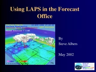
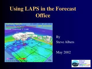
Using LAPS in the Forecast Office. By Steve Albers May 2002. LAPS. A system designed to: Exploit all available data sources Create analyzed and forecast grids Build products for specific forecast applications Use advanced display technology …All within the local weather office.

Using LAPS in the Forecast Office
E N D
Presentation Transcript
Using LAPS in the Forecast Office By Steve Albers May 2002
LAPS A system designed to: • Exploit all available data sources • Create analyzed and forecast grids • Build products for specific forecast applications • Use advanced display technology …All within the local weather office
“THE CONCEPT OF THE LOCAL DATA BASE IS CENTRAL TO FUTURE OPERATIONS…THE MOST COMPLETE DATA SETS WILL ONLY BE AVAILABLE TO THE LOCAL WFO. THE NEW OBSERVING SYSTEMS ARE DESIGNED TO PROVIDE INTEGRATED 3-D DEPICTIONS OF THE RAPIDLY CHANGING STATE OF THE ENVIRONMENT.” -Strategic plan for the modernization and associated restructuring of the National Weather Service
LAPS Grid • LAPS Grid (in AWIPS) • Hourly Time Cycle • Horizontal Resolution = 10 km • Vertical Resolution = 50 mb • Size: 61 x 61 x 21
LAPSDataSources The blue colored data are currently used in AWIPS LAPS. The other data are used in the "full-blown" LAPS and can potentially be added to AWIPS/LAPS if the data becomes available.
Local Surface Data • Local Data may be defined as that data not entering into the National Database • Sources • Highway Departments • Many States with full or partial networks • Agricultural Networks • State run, sometimes private • Universities and Other Schools • Experimental observations • Private Industry • Environmental monitoring • State and Federal Agencies • RAWS
Problems with Local Data • Poor Maintenance • Poor Communications • Poor Calibration Result ----------------> Inaccurate, Irregular, Observations
Multi-layered Quality Control • Gross Error Checks • RoughClimatologicalEstimates • Station Blacklist • Dynamical Models • Use of meso-beta models • Standard Deviation Check • Statistical Models (Kalman Filter) • Buddy Checking
Standard Deviation Check • Compute Standard Deviation of observations-background • Remove outliers • Now adjustable via namelist
Kalman QC Scheme FUTURE Upgrade to AWIPS/LAPS QC • Adaptable to small workstations • Accommodates models of varying complexity • Model error is a dynamic quantity within the filter, thus the scheme adjusts as model skill varies
AWIPS 5.1.2 LAPS Improvements: • Wind Profiler Ingest restored • QC threshold tightened • Surface Stations • More local (LDAD) station data • Improved QC of MSLP
AWIPS 5.2.1 LAPS Improvements: • Surface Analysis • Improved Successive Correction considers instrument and background errors • Works with uneven station spacing and terrain • Reduction of bulls-eye effects (that had occurred even with valid stations) • Improved Surface Pressure Consistency • MSLP • Reduced • Unreduced (terrain following)
AWIPS 5.2.2 LAPS Improvements: • Additional Backgrounds such as AVN • Supports LAPS in Alaska, Pacific • Domain Relocatability • Surface Analysis • Improved fit between obs and analysis • Corrected “theta check” for temperature analysis at high elevation sites • Stability Indices added • Wet Bulb Zero, K, TT, Showalter, LCL
Candidate Future Improvements: • GUI • Domain Resizability • Graphical Product Monitor • Surface Obs QC • Turning on Kalman Filter QC (sfc_qc.exe) • Tighten T, Td QC checks • Allow namelist adjustment of QC checks • Handling of surface stations with known bias
Candidate Future Improvements (cont): • Surface Analysis • Land/Sea weighting to help with coastline effects • Adjustment of reduced pressure height • Other Background Models • Hi-res Eta? • Improved use of radar data • Multiple radars? • Wideband Level-II data? • Sub-cloud evaporation • Doppler radial velocities
Candidate Future Improvements (cont.) • Use of visible & 3.9u satellite in cloud analysis • LI/CAPE/CIN with different parcels in boundary layer • New (Bunkers) method for computing storm motions feeding to helicity determination • Wind profiler • Include obs from just outside the domain • Implies restructuring wind analysis • ACARS • Forecast Model (Hot-Start MM5)
Sources of LAPS Information • The LAPS homepage http://laps.fsl.noaa.gov provides access to many links including: • What is in AWIPS LAPS? http://laps.fsl.noaa.gov/LAPB/AWIPS_WFO_page.htm
Analysis Information LAPS analysis discussions are near the bottom of: http://laps.fsl.noaa.gov/presentations/presentations.html Especially noteworthy are the links for • Satellite Meteorology • Analyses: Temperature, Wind, and Clouds/Precip. • Modeling and Visualization • A Collection of Case Studies
3-D Temperature • Interpolate from model (RUC) • Insert RAOB, RASS, and ACARS if available • 3-Dimensional weighting used • Insert surface temperature and blend upward • depending on stability and elevation • Surface temperature analysis depends on • METARS, Buoys, and LDAD • Gradients adjusted by IR temperature
3-D Clouds • Preliminary analysis from vertical “soundings” derived from METARS and PIREPS • IR used to determine cloud top (using temperature field) • Radar data inserted (3-D if available) • Visible satellite can be used
LAPS 3-D Water Vapor (Specific Humidity) Analysis • Interpolates background field from synoptic-scale model forecast • QCs against LAPS temperature field (eliminates possible supersaturation) • Assimilates RAOB data • Assimilates boundary layer moisture from LAPS Sfc Td analysis • Scales moisture profile (entire profile excluding boundary layer) to agree with derived GOES TPW (processed at NESDIS) • Scales moisture profile at two levels to agree with GOES sounder radiances (channels 10, 11, 12). The levels are 700-500 hPa, and above 500 • Saturates where there are analyzed clouds • Performs final QC against supersaturation
Case Study Example An example of the use of LAPS in convective event 14 May 1999 Location: DEN-BOU WFO
Quote from the Field "...for the hourly LAPS soundings, you can go to interactive skew-T, and loop the editable soundings from one hour to the next, and get a more accurate idea of how various parameters are changing on an hourly basis...nice. We continue to find considerable use of the LAPS data (including soundings) for short-term convective forecasting."
Case Study Example • On 14 May, moisture is in place. A line of storms develops along the foothills around noon LT (1800 UTC) and moves east. LAPS used to diagnose potential for severe development. A Tornado Watch issued by ~1900 UTC for portions of eastern CO and nearby areas. • A brief tornado did form in far eastern CO west of GLD around 0000 UTC the 15th. Other tornadoes occurred later near GLD.
Dewpoint max appears near CAPE max, but between METARS 2100 UTC
Examine soundings near CAPE max at points B, E and F 2100 UTC
LAPS & RUC sounding comparison at point E (CAPE Max) 2100 UTC
CAPE Maximum persists in same area 2200 UTC
CIN minimum in area of CAPE max 2200 UTC
Convergence and Equivalent Potential Temperature are co-located 2100 UTC
How does LAPS sfc divergence compare to that of the RUC? Similar over the plains. 2100 UTC
Case Study Example (cont.) • The next images show a series of LAPS soundings from near LBF illustrating some dramatic changes in the moisture aloft. Why does this occur?
LAPS sounding near LBF 1600 UTC