Download
1 / 23
230 likes | 316 Views
How insurance affects the demand for medical care. Richard Hirth. Ideal health insurance structure. Insurer observes health state Cash payment based on health state

E N D
How insurance affects the demand for medical care Richard Hirth
Ideal health insurance structure • Insurer observes health state • Cash payment based on health state • Set to equate marginal utility of income across all possible health states; thus, large payments made (income transfers) for health states in which expensive care is highly productive • Insured can spend the payment on whatever they please; thus, no distortion of prices • Not feasible because health state cannot be perfectly observed; thus, insurance contracts “pay off” by lowering price of care and dollar value of the pay off depends on amount of care
How insurance affects the demand for medical care Demand is influenced by incentives created by the insurance- induced reduction in the price of care to the consumer “Traditional” FFS insurance: Can impose cost-sharing Does not directly “manage” care (UR, selective contracting, provider incentives) Examining the potential and limitations of traditional insurance helps clarify the rationale for managed care
A. Many HI plans (both traditional and managed) employ copayments (coinsurance) Enrollees pay a fraction of the price of care Encourages some cost-sensitivity when seeking care or choosing a provider Higher copayment more incentive to remain cost-conscious, but more financial risk. Thus, the fundamental trade-off in traditional insurance is incentives versus risk sharing.
Patient pays cpm for a unit of care Insurer pays (1-c) pm Slides the consumer down her demand curve from A to B. Consumer behaves as if the price of care had fallen to cpm. For coinsurance rate c: P A • Pm B cPm • D Q Figure 1
Translating “sliding down” the uninsured D curve into a “with insurance” D curve: 1) Start with the no insurance D curve. This shows which P (actually paid by the consumer) leads to any particular Q. 2) For each Q, find the P where out-of-pocket price with insurance = P on the no insurance D curve Uninsured consumer buys Q=10 units at P=$20 If C=.2, she would buy Q=10 at P=$100 This is one point on the insured D curve 3) Connect the “with insurance” Ps and Qs to get the “with insurance” D curve
Translating “sliding down” the uninsured D curve into a “with insurance” D curve (cont’d.): P • $100 D with insurance • $20 D no insurance 10 Figure 2
An alternative way of translating an uninsured D curve to an insured D curve: Uninsured D curve represents 100% coinsurance (c=1) With full insurance (c=0), demand for care would be perfectly price inelastic (vertical) D curves with 0<c<1 can be determined by rotating the no insurance D curve around the Q intercept towards the full insurance D curve. Insured D curve becomes steeper (less P elastic) as the copayment falls. If health care markets are not perfectly competitive, how will insurance influence prices and profits?
Creating a “with insurance” D curve P D full insurance • $100 Dc = .2 D no insurance • $20 A 10 15 Q Figure 3
B. Indemnity insurance pays a fixed $ amount per unit of care To see the effect on the D curve: • Suppose an uninsured consumer buys 10 units of care at p=$40 • Indemnity pays $80 per unit regardless of the price of care • If p=$120, consumer faces out-of-pocket p=$40 and demands Q=10; • Insured D curve shifts up by the amount of the indemnity payment How do incentives to “price shop” differ under an indemnity Policy vs. a policy with coinsurance?
B. Indemnity insurance pays a fixed $ amount per unit of care (cont’d): P $120 $100 D indemnity $40 D no insurance $20 10 20 Q Figure 4
C.Deductibles imply that the consumer faces different prices at different quantities: e.g., $500 deductible and 20% coinsurance; p=$100 Effects of deductible depend on the level of illness: • For minor illness, deductible > expenditures, so the consumer faces the full price of $100 • For serious illness, expenditure > deductible, so the price of the marginal unit of care is only $20 Effects of deductibles also depend on time (January 1 vs. December 31) and health status
C.Deductibles imply that the consumer faces different prices at different quantities (cont’d.): P D Minor illness D Severe illness $100 $20 Out-of-pocket price 5 Q Figure 5
D. Maximum payment provisions are the opposite of deductibles If policy limits coverage to $100,000 (or to 30 days of inpatient care), I face a low price for small amounts of care, but a high price for high levels of care
Why should we care about the demand for Medical care? (or “Demand” vs. “Need”) • If we’re concerned about utilization by a population, it is important to understand how demand is determined • A policy analysis based on the concept of ‘demand” can • yield different results than one based on the concept of • “need” (“need” = amount of care that “experts” believe • some person or population should have)
Several policies have been shaped by need-based analyses: 1) Hill-Burton Act Subsidies for hospital construction predicated on a standard of 4.5 beds per 1000 population Since “need” is independent of price, it is represented by the vertical line at 4.5 beds/1000 Residents of an area with D1 would have to be paid to consume as much inpatient care as they “need;” subsidies to build capacity to 4.5/1000 would be wasted
Hill-Burton Act (cont’d.) Residents of an area with D2 would only consume what they “need” at a price of p* “need” P* D1 D2 4.5 beds/1000 pop. Figure 6
Hill-Burton Act (cont’d.) 2) Health workforce policies Step 1: Forecasts of physicians needed to serve the population (based on expected #s of people with various diseases and assumptions about optimal care) Step 2: Compare to actual # of physicians (given existing trends) to calculate future surplus or shortage These forecasts were important determinants of policies such as subsidization of medical schools In response to errors generated by a need-based approach, recent workforce forecasts have been based at least partly on the concept of demand
The moral of the story: Even if you believe that people’s preferences (as expressed through D curves) should be over- ridden in favor of expert opinion about “need,” you’ll still need to know about the determinants of D to get them to consume what you think they need
Empirical studies of the demand for medical care P elasticity of D for medical care determines how insurance affects the quantity of care demanded: Price faced by the consumer is pc = pm*c 1% increase in either pm or c results in a 1% increase in out-of-pocket price Many attempts to estimate the price elasticity of D: • Estimates all over the place (0 to -3)
Methodological limitations: Need to observe consumers who face different Ps • Same person, P changes over time • Different people facing different Ps at one point in time Studies often use insurance coverage as the source of P variation Biased elasticity estimates (people who expect to consume more medical care enroll in more generous health plans, causing the observed relationship between insurance coverage and utilization to include both the pure response to price and a “selection effect”)
RAND Health Insurance Experiment (HIE) Patients randomly assigned to different levels of coverage to allow estimation of the pure price effect 6 sites including one with a staff model HMO Enrollment 1974-77; 3-5 year follow-up C varied from 0 to 0.95, $1000 out-of-pocket maximum
RAND HIE: Key results (see handout for details): Cost-sharing matters (expenses fell 30% when c went from 0 to 0.95) Few health consequences of marginal utilization P elasticity of demand overall in the range of -0.1 to -0.2 Income elasticity 0.2 for outpatient, 0 for inpatient Cost-sharing reduced utilization of care deemed “effective” as much as care deemed “ineffective;” are patients good rationers?