Multi-layer Orthogonal Codebook for Image Classification
Multi-layer Orthogonal Codebook for Image Classification. Presented by Xia Li. Outline . Introduction Motivation Related work Multi-layer orthogonal codebook Experiments Conclusion. Image Classification. Sampling:.

Multi-layer Orthogonal Codebook for Image Classification
E N D
Presentation Transcript
Multi-layer Orthogonal Codebook for Image Classification Presented by Xia Li
Outline • Introduction • Motivation • Related work • Multi-layer orthogonal codebook • Experiments • Conclusion
Image Classification Sampling: • For object categorization, dense sampling offers better coverage. [Nowak, Jurie & Triggs, ECCV 2006] Sparse, at interest points Dense, uniformly Descriptor: • Use orientation histograms within sub-patches to build 4*4*8=128 dim SIFT descriptor vector. [David Lowe, 1999, 2004] Image credits: F-F. Li, E. Nowak, J. Sivic
Image Classification • Visual codebook construction • Supervised vs. Unsupervised clustering • k-means (typical choice), agglomerative clustering, mean-shift,… • Vector Quantization via clustering • Let cluster centers be the prototype “visual words” • Assign the closest cluster center to each new image patch descriptor. Descriptor space Image credits: K. Grauman, B. Leibe
Image Classification Bags of visual words • Represent entire image based on its distribution (histogram) of word occurrences. • Analogous to bag of words representation used for documents classification/retrieval. Image credit: Fei-Fei Li
Image Classification [S. Lazebnik, C. Schmid, and J. Ponce, CVPR 2006] Image credit: S. Lazebnik
Image Classification • Histogram intersection kernel: • Linear kernel: Image credit: S. Lazebnik
Image Classification [S. Lazebnik, C. Schmid, and J. Ponce, CVPR 2006] Image credit: S. Lazebnik
Motivation • Codebook quality • Feature type • Codebook creation • Algorithm e.g. K-Means • Distance metric e.g. L2 • Number of words • Quantization process • Hard quantization: only one word is assigned for each descriptor • Soft quantization: multi-words may be assigned for each descriptor
Motivation • Quantization error • The Euclidean squared distance between a descriptor vector and its mapped visual word Hard quantization leads to large error Effects of descriptor hard quantization – Severe drop in descriptor discriminative power. A scatter plot of descriptor discriminative power before and after quantization. The display is in logarithmic scale in both axes. O. Boiman, E. Shechtman, M. Irani, CVPR 2008
Motivation • Codebook size is an important factor for applications that need efficiency • Simply enlarging codebook size can reduce overall quantization error • but cannot guarantee every descriptor got reduced error The right column is the percentage of descriptors whose quantization error is reduced when codebook size grows
Motivation • Good codebook for classification • Small individual quantization error -> discriminative • Compact in size • Contradict in some extent • Overemphasizing on discriminative ability may increase the size of dictionary and weaken its generalization ability • Over-compressing to a dictionary will more or less lose the information and its discriminative power • Find a balance! [X. Lian, Z. Li, C. Wang, B. lu, and L. Zhang, CVPR 2010]
Related Work • No quantization • NBNN [6] • Supervised codebook • Probabilistic models [5] • Unsupervised codebook • Kernel codebook [2] • Sparse coding [3] • Locality-constrained linear coding [4]
Multi-layer Orthogonal Codebook (MOC) • Use standard K-Means to keep efficiency or any other clustering algorithm can be adopted • Build codebook from residues to reduce quantization errors explicitly
MOC Creation • First layer codebook • K-Means • Residue: N is the number of descriptors randomly sampled to build the codebook, di is one of the descriptors.
MOC Creation • Orthogonal residue: • Second layer codebook • K-Means Third layer …
Vector Quantization • How to use MOC? • Kernel fusion: use them separately • Compute the kernels based on each layer codebook separately • Let the final kernel to be the combination of multiple kernels • Soft weighting: adjust weight for words from different layers individually for each descriptor • Select the nearest word on each layer codebook for a descriptor • Use the selected words from all layers to reconstruct that descriptor and minimize reconstruction error
Hard Quantization and Kernel Fusion (HQKF) • Hard quantization on each layer • average pooling: descriptors in the m-th sub-region, totally M sub-regions on an image, histogram for m-th sub-region is • Histogram intersection kernel …… • Linear combine kernel values from each codebook
Soft Weighting (SW) • Weighting words for each descriptor • Max pooling • Linear kernel K is codebook size
Soft Weighting (SW-NN) • To further consider the relationships between words from multi-layers • Select 2 or more nearest words on each layer codebook, and then weighting them to reconstruct the descriptor • Each descriptor is more accurately represented by multiple words on each layer • The correlation between similar descriptors by sharing words is captured d2 d1 [J. Wang, J. Yang, K. Yu, F. Lv, T. Huang, Y. Gong, CVPR 2010]
Experiment • Single feature type: SIFT • 16*16 pixel patches densely sampled over a grid with spacing of 6 pixels • Spatial pyramid layer: • 21=16+4+1 sub-regions at three resolution level • Clustering method on each layer: K-Means
Datasets • Caltech-101 • 101 categories, 31-800 images per category • 15 Scenes • 15 scenes, 4485 images
Quantization Error • Quantization error is reduced more effectively by MOC compared with simply enlarging codebook size • Experiment is done on Caltech101 The right column is the percentage of descriptors whose quantization error is reduced when codebook changes
Codebook Size • Classification accuracy comparisons with single layer codebook Comparison with single codebook (Caltech101). 2-layer codebook has the same size on each layer which is also the same size as the single layer codebook.
Comparisons with existing methods • Classification accuracy comparisons with existing methods Listed methods all used single type descriptor *only LLC used HoG instead of SIFT, we repeated their method with the type of descriptors we use, result is 71.63±1.2
Conclusion • Compared with existing methods, the proposed approach has the following merits: • 1) No complex algorithm and easy to implement. • 2) No time-consuming learning or clustering stage. Able to be applied on large scale computer vision systems. • 3) Even more efficient than traditional K-Means clustering. • 4) Explicit residue minimization to explore discriminative power of descriptors. • 5) The basic idea can be combined with many state-of-the-art methods.
References • [1] S. Lazebnik, C. Schmid, and J. Ponce, “Beyondbags of features: Spatial pyramid matching for recognizingnatural scene categories,”CVPR, pp. 2169 –2178, 2006. • [2] J. Gemert, J. Geusebroek, C. Veenman, and A. Smeulders, “Kernel codebooks for scene categorization,”ECCV, pp. 696-709, 2008. • [3] J. Yang, K. Yu, Y. Gong, and T. Huang, “Linear spatial pyramid matching using sparse coding for image classification,”CVPR, pp. 1794-1801, 2009. • [4] J. Wang, J. Yang, K. Yu, F. Lv, T. Huang, and Y. Gong, “Locality-constrained linear coding for image classification,”CVPR, pp. 3360-3367, 2010. • [5] X. Lian, Z. Li, C. Wang, B. Lu, and L. Zhang, “Probabilistic models for supervised dictionary learning,” CVPR, pp. 2305-2312, 2010. • [6] O. Boiman, I. Rehovot, E. Shechtman, and M. Irani, “In defense of nearest-neighbor based image classification,”CVPR, pp. 1-8, 2008.
Codebook Size • Different size combination on 2-layer MOC Caltech101: The X-axis is the size of the 1st layer codebook Different colors represent the size of the 2nd layer codebook