Schema Refinement, Normalization, and Tuning
Schema Refinement, Normalization, and Tuning. Design Steps. The design steps: 1. Real-World 2. ER model 3. Relational Schema 4. Better relational Schema 5. Relational DBMS

Schema Refinement, Normalization, and Tuning
E N D
Presentation Transcript
Design Steps • The design steps: 1. Real-World 2. ER model 3. Relational Schema 4. Better relational Schema 5. Relational DBMS • Step (3) to step (4) is based on a “design theory” for relations and is called “normalization”. It is important for two reasons: • Automatic mappings from ER to relations may not produce the best relational design possible. • Database designers may go directly from (1) to (3), in which case, the relational design can be really bad.
The Evils of Redundancy • Redundancyis the root of several problems associated with relational schemas: • redundant storage, insert/delete/update anomalies • Consider relation obtained from Hourly_Emps: • Hourly_Emps (ssn, name, lot, rating, hrly_wages, hrs_worked) • Notation: We will denote this relation schema by listing the attributes: SNLRWH • This is really the set of attributes {S,N,L,R,W,H}. • Sometimes, we will refer to all attributes of a relation by using the relation name. (e.g., Hourly_Emps for SNLRWH)
Example • Problems due to R W : • Update anomaly: Can we change W in just the 1st tuple of SNLRWH? • Insertion anomaly: What if we want to insert a employee and don’t know the hourly wage for his rating? • Deletion anomaly: If we delete all employees with rating 5, we lose the information about the wage for rating 5!
Refinements • Integrity constraints, in particularfunctional dependencies, can be used to identify schemas with such problems and to suggest refinements. • Main refinement technique: decomposition (replacing ABCD with, say, AB and BCD, or ACD and ABD). • Decomposition should be used judiciously: • Is there reason to decompose a relation? • What problems (if any) does the decomposition cause?
Functional Dependencies (FDs) • A functional dependencyX Y holds over relation R if, for every allowable instance r of R: • i.e., given two tuples in r, if the X values agree, then the Y values must also agree. (X and Y are sets of attributes.) • K is a key for relation R if: 1. K determines all attributes of R. 2. For no proper subset of K is (1) true. • If K satisfies only (1), then K is a superkey. • K is a candidate key for R means that K R • However, K R does not require K to be minimal!
Example • Consider relation Hourly_Emps: • Hourly_Emps (ssn, name, lot, rating, hrly_wages, hrs_worked) • FD is a key: • ssn is the key • S SNLRWH • FDs give more detail than the mere assertion of a key. • rating determines hrly_wages • R W
Who Determines Keys/FDs? • An FD is a statement about all allowable relations. • Must be identified based on semantics of application. • Given some allowable instance r1 of R, we can check if it violates some FD f, but we cannot tell if f holds over R! • We can define a relation schema with a single key K. • Then the only FD asserted are K A for every attribute A. • Or, we can assert some FDs and deduce one or more keys or other FDs.
Reasoning About FDs • Given some FDs, we can usually infer additional FDs: • ssn did, did lot implies ssn lot • An FD f is implied bya set of FDs F if f holds whenever all FDs in F hold. • F+ = closure of F is the set of all FDs that are implied by F. • Armstrong’s Axioms (X, Y, Z are sets of attributes): • Reflexivity: If Y X, then X Y • Augmentation: If X Y, then XZ YZ for any Z • Transitivity: If X Y and Y Z, then X Z • These are sound and completeinference rules for FDs!
Reasoning About FDs (Cont.) • Couple of additional rules (that follow from AA): • Union: If X Y and X Z, then X YZ • Decomposition: If X YZ, then X Y and X Z • Proof of Union: • X Y (given) • X XY (augmentation using X) • X Z (given) • XY YZ (augmentation) • X YZ (transitivity)
Reasoning About FDs (Cont.) • Example: Contracts(cid,sid,jid,did,pid,qty,value) • C is the key: C CSJDPQV • Project purchases each part using single contract: JP C • Dept purchases at most one part from a supplier: SD P • JP C, C CSJDPQV imply JP CSJDPQV • SD P implies SDJ JP • SDJ JP, JP CSJDPQV imply SDJ CSJDPQV
Reasoning About FDs (Cont.) • Computing the closure of a set of FDs can be expensive. (Size of closure is exponential in # attrs!) • Typically, we just want to check if a given FD X Y is in the closure of a set of FDs F. An efficient check: • Compute attribute closureof X (denoted X+) wrt F: • Set of all attributes A such that X A is in • There is a linear time algorithm to compute this. • Check if Y is in X+ • Does F = {A B, B C, C D E } imply A E? • i.e, is A E in the closure F+ ? Equivalently, is E in A+ ?
Algorithm to Compute Attribute Closure • Define Y+ = closure of Y. • Basis: Y+ = Y • Induction: If X Y+, and X A is a given FD, then add A to Y+ • End when Y+ cannot be changed. Then Y functionally determines all members of Y+, and no other attributes.
Example • A B, BC D • A+ = AB • C+ = C • (AC)+ = ABCD • Thus, AC is a key.
Finding All Implied FDs • Motivation: Suppose we have a relation ABCD with some FDs F. If we decide to decompose ABCD into ABC and AD, what are the FDs for ABC, AD? • Example: F = AB C, C D, D A. It looks like just AB C holds in ABC, but in fact C A follows from F and applies to relation ABC. • Problem is exponential in worst case. • Algorithm to find F+: • For each set of attributes X of R, compute X+.
Example • F = AB C, C D, D A. What FDs follow? • A+ = A; B+ = B (nothing) • C+ = ACD (add C A) • D+ = AD (nothing new) • (AB)+ = ABCD (add AB D; skip all supersets of AB). • (BC)+ = ABCD (nothing new; skip all supersets of BC). • (BD)+ = ABCD (add BD C; skip all supersets of BD). • (AC)+ = ACD; (AD)+ = AD; (CD)+ = ACD (nothing new). • (ACD)+ = ACD (nothing new). • All other sets contain AB, BC, or BD, so skip. • Thus, the only interesting FDs that follow from F are: • C A, AB D, BD C.
Projection of set of FDs • If R is decomposed into X, ... projection of F onto X (denoted FX ) is the set of FDs U V in F+(closure of F )such that U, V are in X. • Using the same example, • R1(ABC): AB C, C A • R2(AD): D A
A BAD Relational Schema An Improved Schema
What’s a Good Design? • Three properties: • No anomalies. • Can reconstruct all original information. • Ability to check all FDs within a single relation. • Role of FDs in detecting redundancy: • Consider a relation R with 3 attributes, ABC. • No FDs hold: There is no redundancy here. • Given A B: Several tuples could have the same A value, and if so, they’ll all have the same B value!
Decomposition of a Relation Scheme • Suppose that relation R contains attributes A1 ... An. A decompositionof R consists of replacing R by two or more relations such that: • Each new relation scheme contains a subset of the attributes of R (and no attributes that do not appear in R), and • Every attribute of R appears as an attribute of one of the new relations. • Intuitively, decomposing R means we will store instances of the relation schemes produced by the decomposition, instead of instances of R. • E.g., Can decompose SNLRWH into SNLRH and RW.
Example Decomposition • Decompositions should be used only when needed. • SNLRWH has FDs S SNLRWH and R W • W values repeatedly associated with R values. Easiest way to fix this is to create a relation RW to store these associations, and to remove W from the main schema: • i.e., we decompose SNLRWH into SNLRH and RW • The information to be stored consists of SNLRWH tuples. If we just store the projections of these tuples onto SNLRH and RW, are there any potential problems that we should be aware of?
Problems with Decompositions • There are three potential problems to consider: • Some queries become more expensive. • e.g., How much did sailor Joe earn? (salary = W*H) • Given instances of the decomposed relations, we may not be able to reconstruct the corresponding instance of the original relation! • Fortunately, not in the SNLRWH example. • Checking some dependencies may require joining the instances of the decomposed relations. • Fortunately, not in the SNLRWH example. • Tradeoff: Must consider these issues vs. redundancy.
Lossless Join Decompositions • Decomposition of R into X and Y is lossless-join w.r.t. a set of FDs F if, for every instance r that satisfies F, “reassembling” X and Y will give R and nothing else. • It is always true that reassembling X and Y gives exactly R or a superset of R. • Definition extended to decomposition into 3 or more relations in a straightforward way. • It is essential that all decompositions used to deal with redundancy be lossless! (Avoids Problem (2).)
More on Lossless Join • The decomposition of R into X and Y is lossless-join wrt F if and only if the closure of F contains: • X Y X, or • X Y Y • In particular, the decomposition of R into UV and R - V is lossless-join if U V holds over R.
Dependency Preserving Decomposition • Consider CSJDPQV, C is key, JP C and SD P. • BCNF decomposition: CSJDQV and SDP • Problem: Checking JP C requires a join! • Dependency preserving decomposition (Intuitive): • If R is decomposed into X, Y and Z, and we enforce the FDs that hold on X, on Y and on Z, then all FDs that were given to hold on R must also hold. (Avoids Problem (3).)
Dependency Preserving Decompositions (Cont.) • Decomposition of R into X and Y is dependencypreserving if (FX union FY ) + = F + • i.e., if we consider only dependencies in the closure F + that can be checked in X without considering Y, and in Y without considering X, these imply all dependencies in F +. • Important to consider F +, not F, in this definition: • ABC, A B, B C, C A, decomposed into AB and BC. • Is this dependency preserving? • Dependency preserving does not imply lossless join: • ABC, A B, decomposed into AB and BC. • And vice-versa! (Example?) Is C A preserved?????
Normal Forms • Returning to the issue of schema refinement, the first question to ask is whether any refinement is needed! • If a relation is in a certain normal form(BCNF, 3NF etc.), it is known that certain kinds of problems are avoided/minimized. This can be used to help us decide whether decomposing the relation will help.
Normal forms Universe of relations 1 NF 2NF 3NF BCNF 4NF 5NF
Boyce-Codd Normal Form (BCNF) • Reln R with FDs F is in BCNF if, for all X A in F+ • A X (called a trivial FD), or • X contains a key for R. • In other words, R is in BCNF if the only non-trivial FDs that hold over R are key constraints. • Why? • Guarantees no redundancy due to FDs. • Guarantees no insert/update/delete anomalies. • Guarantees no loss of information. • But … • May destroy the ability to check FDs within a single relation
Example • Consider relation Beers(name, manf, manfAddr). • FDs = name manf, manf manfAddr • Only key is name. • manf manfAddr violates BCNF with a left side unrelated to any key. • Redundancy (every manf has the same manfAddr) • Update anomalies (if manf moves, all manfAddr in ALL tuples) • Deletion anomalies (deleting all beers produced by a particular manf will lose info on manf and manfAddr) • Not in BCNF.
Third Normal Form (3NF) • Reln R with FDs F is in 3NF if, for all X A in F+ • A X (called a trivial FD), or • X contains a key for R, or • A is part of some minimal key for R. • If R is in BCNF, obviously in 3NF. • If R is in 3NF, some redundancy is possible. It is a compromise, used when BCNF not achievable (e.g., no ``good’’ decomp, or performance considerations).
What Does 3NF Achieve? • If 3NF violated by X A, one of the following holds: • X is a subset of some key K • We store (X, A) pairs redundantly. • X is not a proper subset of any key. • There is a chain of FDs K X A, which means that we cannot associate an X value with a K value unless we also associate an A value with an X value. • But: even if reln is in 3NF, these problems could arise. • e.g., Reserves SBDC, S C, C S is in 3NF, but for each reservation of sailor S, same (S, C) pair is stored. • Thus, 3NF is indeed a compromise relative to BCNF.
Decomposition into BCNF • Consider relation R with FDs F. If X Y violates BCNF, • Expand left side to include X+. • Decompose R into (R - X+) U X and X+. • Find the FDs for the decomposed relations. • Repeated application of this idea will give us a collection of relations that are in BCNF; lossless join decomposition, and guaranteed to terminate. • In general, several dependencies may cause violation of BCNF. The order in which we ``deal with’’ them could lead to very different sets of relations!
Example • R(A, C, B, D, E) • F = A B, A E, C D • Since AC is a key, not in BCNF. • Pick A B for decomposition. • Expand left side: A B E • Decomposed relations: R1(A,B,E) and R2(A,C,D). • Projected FDs (skipping a lot of work …) • R1: A B, A E • R2: C D
Example (Cont) • BCNF violations? • For R1, A is key and all left sides are superkeys. • For R2, AC is key, and C D violates BCNF. • Decompose R2 • R3(C,D) • R4(A,C) • Resulting relations are all in BCNF. • R1(A,B,E) • R3(C,D) • R4(A,C)
BCNF and Dependency Preservation • The example decomposition is dependency preserving! • In general, there may not be a dependency preserving decomposition into BCNF. • e.g., CSZ, CS Z, Z C • Can’t decompose while preserving 1st FD; not in BCNF.
Decomposition into 3NF • Obviously, the algorithm for lossless join decomp into BCNF can be used to obtain a lossless join decomp (not necessarily dependency preserving) into 3NF (typically, can stop earlier). • There exists an algorithm that guarantees a lossless-join and dependency preserving decomp in 3NF. No such algorithm for BCNF!
Decomposition into 3NF (Cont) • To ensure dependency preservation, one idea: • If X Y is not preserved, add relation XY. • Problem is that XY may violate 3NF! e.g., consider the addition of CJP to `preserve’ JP C. What if we also have J C ? • Refinement: Instead of the given set of FDs F, use a minimal cover for F.
Minimal Cover for a Set of FDs • Minimal coverG for a set of FDs F: • Closure of F = closure of G. • Right hand side of each FD in G is a single attribute. • If we modify G by deleting an FD or by deleting attributes from an FD in G, the closure changes. • Intuitively, every FD in G is needed, and ``as small as possible’’ in order to get the same closure as F. • e.g., A B, ABCD E, EF GH, ACDF EG has the following minimal cover: • A B, ACD E, EF G and EF H • M.C. ® Lossless-Join, Dep. Pres. Decomp!!!
Determining a minimal cover of F • Obtain a collection G of equivalent FDs with a single attribute on the right side (decomposition axiom) • For each FD in G, check each attribute in the LHS to see if it can be deleted while preserving equivalence to F+ • Check each remaining FD in G to see if it can be deleted while preserving equivalence to F+
Dependency Preserving Decomp into 3NF • Let R be a relation, F a set of FDs that is a minimal cover, R1, …, Rn be a lossless –join decomp of R. Suppose each Ri is in 3NF, and Fi denote the projection of F onto the attributes of Ri • Let N be the dependencies in F that are not preserved • For each FD X A in N, create a relation XA and add it to the decomposition of R
Summary of Schema Refinement • If a relation is in BCNF, it is free of redundancies that can be detected using FDs. Thus, trying to ensure that all relations are in BCNF is a good heuristic. • If a relation is not in BCNF, we can try to decompose it into a collection of BCNF relations. • Must consider whether all FDs are preserved. If a lossless-join, dependency preserving decomposition into BCNF is not possible (or unsuitable, given typical queries), should consider decomposition into 3NF. • Decompositions should be carried out and/or re-examined while keeping performance requirements in mind.
Settings: lineitem ( L_ORDERKEY, L_PARTKEY , L_SUPPKEY, L_LINENUMBER, L_QUANTITY, L_EXTENDEDPRICE , L_DISCOUNT, L_TAX , L_RETURNFLAG, L_LINESTATUS , L_SHIPDATE, L_COMMITDATE, L_RECEIPTDATE, L_SHIPINSTRUCT , L_SHIPMODE , L_COMMENT ); region( R_REGIONKEY, R_NAME, R_COMMENT ); nation( N_NATIONKEY, N_NAME, N_REGIONKEY, N_COMMENT,); supplier( S_SUPPKEY, S_NAME, S_ADDRESS, S_NATIONKEY, S_PHONE, S_ACCTBAL, S_COMMENT); 600000 rows in lineitem, 25 nations, 5 regions, 500 suppliers Denormalizing -- data
Denormalizing -- transactions lineitemdenormalized ( L_ORDERKEY, L_PARTKEY , L_SUPPKEY, L_LINENUMBER, L_QUANTITY, L_EXTENDEDPRICE , L_DISCOUNT, L_TAX , L_RETURNFLAG, L_LINESTATUS , L_SHIPDATE, L_COMMITDATE, L_RECEIPTDATE, L_SHIPINSTRUCT , L_SHIPMODE , L_COMMENT, L_REGIONNAME); • 600000 rows in lineitemdenormalized • Cold Buffer • Dual Pentium II (450MHz, 512Kb), 512 Mb RAM, 3x18Gb drives (10000RPM), Windows 2000.
Queries on Normalized vs. Denormalized Schemas Queries: select L_ORDERKEY, L_PARTKEY, L_SUPPKEY, L_LINENUMBER, L_QUANTITY, L_EXTENDEDPRICE, L_DISCOUNT, L_TAX, L_RETURNFLAG, L_LINESTATUS, L_SHIPDATE, L_COMMITDATE, L_RECEIPTDATE, L_SHIPINSTRUCT, L_SHIPMODE, L_COMMENT, R_NAME from LINEITEM, REGION, SUPPLIER, NATION where L_SUPPKEY = S_SUPPKEY and S_NATIONKEY = N_NATIONKEY and N_REGIONKEY = R_REGIONKEY and R_NAME = 'EUROPE'; select L_ORDERKEY, L_PARTKEY, L_SUPPKEY, L_LINENUMBER, L_QUANTITY, L_EXTENDEDPRICE, L_DISCOUNT, L_TAX, L_RETURNFLAG, L_LINESTATUS, L_SHIPDATE, L_COMMITDATE, L_RECEIPTDATE, L_SHIPINSTRUCT, L_SHIPMODE, L_COMMENT, L_REGIONNAME from LINEITEMDENORMALIZED where L_REGIONNAME = 'EUROPE';
TPC-H schema Query: find all lineitems whose supplier is in Europe. With a normalized schema this query is a 4-way join. If we denormalize lineitem and add the name of the region for each lineitem (foreign key denormalization) throughput improves 30% Denormalization
Schema Tuning Rule of Thumb: If ABC is normalized, and AB and AC are also normalized, then use ABC, unless: • Queries very rarely access ABC, but AB or AC (80% of the time) • Attribute B or C values are large.
Example • Schema 1: • R1(bond_ID, issue_date, maturity, …) • R2(bond_ID, date, price) • Schema 2: • R1(bond_ID, issue_date, maturity, today_price, yesterday_proce,…,10dayago_price) • R2(bond_ID, date, price)