Download

1 / 78
780 likes | 832 Views
Learn differentiation rules to calculate derivatives effortlessly for polynomials, exponential, and more functions. Understand how to find tangent and normal lines for curves.

E N D
3 DIFFERENTIATION RULES
DIFFERENTIATION RULES • We have: • Seen how to interpret derivatives as slopes and rates of change • Seen how to estimate derivatives of functions given by tables of values • Learned how to graph derivatives of functions that are defined graphically • Used the definition of a derivative to calculate the derivatives of functions defined by formulas
DIFFERENTIATION RULES • However, it would be tedious if we always had to use the definition. • So, in this chapter, we develop rules for finding derivatives without having to use the definition directly.
DIFFERENTIATION RULES • These differentiation rules enable us to calculate with relative ease the derivatives of: • Polynomials • Rational functions • Algebraic functions • Exponential and logarithmic functions • Trigonometric and inverse trigonometric functions
DIFFERENTIATION RULES • We then use these rules to solve problems involving rates of change and the approximation of functions.
DIFFERENTIATION RULES 3.1Derivatives of Polynomials and Exponential Functions • In this section, we will learn: • How to differentiate constant functions, power functions, • polynomials, and exponential functions.
CONSTANT FUNCTION • Let’s start with the simplest of all functions—the constant function f(x) = c.
CONSTANT FUNCTION • The graph of this function is the horizontal line y = c, which has slope 0. • So, we must have f’(x)=0.
CONSTANT FUNCTION • A formal proof—from the definition of a derivative—is also easy.
DERIVATIVE • In Leibniz notation, we write this rule as follows.
POWER FUNCTIONS • We next look at the functions f(x) = xn, where n is a positive integer.
POWER FUNCTIONS Equation 1 • If n = 1, the graph of f(x)= x is the line y = x, which has slope 1. • So, • You can also verify Equation 1 from the definition of a derivative.
POWER FUNCTIONS Equation 2 • We have already investigated the cases n =2 and n =3. • In fact, in Section 2.8, we found that:
POWER FUNCTIONS • For n = 4 we find the derivative of f(x)= x4 as follows:
POWER FUNCTIONS Equation 3 • Thus,
POWER FUNCTIONS • Comparing Equations 1, 2, and 3, we see a pattern emerging. • It seems to be a reasonable guess that, when n is a positive integer, (d/dx)(xn)= nxn -1. • This turns out to be true.
POWER RULE • If n is a positive integer, then
POWER RULE Proof 1 • The formula can be verified simply by multiplying out the right-hand side (or by summing the second factor as a geometric series).
POWER RULE Proof 1 • If f(x)= xn, we can use Equation 5 in Section 2.7 for f’(a) and the previous equation to write:
POWER RULE Proof 2 • In finding the derivative of x4,we had to expand (x + h)4. • Here, we need to expand (x + h)n . • To do so, weuse the Binomial Theorem—as follows.
POWER RULE Proof 2 • This is because every term except the first has has a factor and therefore approaches 0.
POWER RULE • We illustrate the Power Rule using various notations in Example 1.
POWER RULE Example 1 • If f(x) = x6, then f’(x) = 6x5 • If y = x1000, then y’ = 1000x999 • If y = t4, then • = 3r2
NEGATIVE INTEGERS • What about power functions with negative integer exponents? • In Exercise 61, we ask you to verify from the definition of a derivative that: • We can rewrite this equation as:
NEGATIVE INTEGERS • So, the Power Rule is true when n = -1. • In fact, we will show in the next section that it holds for all negative integers.
FRACTIONS • What if the exponent is a fraction? • In Example 3 in Section 2.8, we found that: • This can be written as:
FRACTIONS • This shows that the Power Rule is true even when n = ½. • In fact, we will show in Section 3.6 that it is true for all real numbers n.
POWER RULE—GENERAL VERSION • If n is any real number, then
POWER RULE Example 2 • Differentiate: • a. • b. • In each case, we rewrite the function as a power of x.
POWER RULE Example 2 a • Since f(x) = x-2, we use the Power Rule with n = -2:
POWER RULE Example 2 b
TANGENT LINES • The Power Rule enables us to find tangent lines without having to resort to the definition of a derivative.
NORMAL LINES • It also enables us to find normal lines. • The normal lineto a curve C at a point P is the line through P that is perpendicular to the tangent line at P. • In the study of optics, one needs to consider the angle between a light ray and the normal line to a lens.
TANGENT AND NORMAL LINES Example 3 • Find equations of the tangent line and normal line to the curve at the point (1, 1). • Illustrate by graphing the curve and these lines.
TANGENT LINE Example 3 • The derivative of is: • So, the slope of the tangent line at (1, 1) is: • Thus, an equation of the tangent line is: or
NORMAL LINE Example 3 • The normal line is perpendicular to the tangent line. • So, its slope is the negative reciprocal of , that is . • Thus, an equation of the normal line is: or
TANGENT AND NORMAL LINES Example 3 • We graph the curve and its tangent line and normal line here.
NEW DERIVATIVES FROM OLD • When new functions are formed from old functions by addition, subtraction, or multiplication by a constant, their derivatives can be calculated in terms of derivatives of the old functions.
NEW DERIVATIVES FROM OLD • In particular, the following formula says that: • The derivative of a constant times a function is the constant times the derivative of the function.
CONSTANT MULTIPLE RULE • If c is a constant and f is a differentiablefunction, then
CONSTANT MULTIPLE RULE Proof • Let g(x) = cf(x). • Then,
NEW DERIVATIVES FROM OLD Example 4
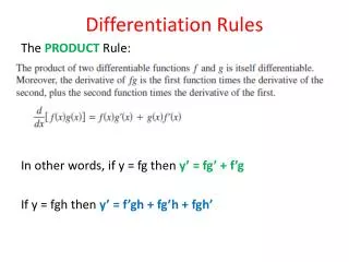
NEW DERIVATIVES FROM OLD • The next rule tells us that the derivative of a sum of functions is the sum of the derivatives.
SUM RULE • If f and g are both differentiable, then
SUM RULE Proof • Let F(x) = f(x) + g(x). Then,
SUM RULE • The Sum Rule can be extended to the sum of any number of functions. • For instance, using this theorem twice, we get:
NEW DERIVATIVES FROM OLD • By writing f - g as f + (-1)g and applying the Sum Rule and the Constant Multiple Rule, we get the following formula.
DIFFERENCE RULE • If f and g are both differentiable, then
NEW DERIVATIVES FROM OLD • The Constant Multiple Rule, the Sum Rule, and the Difference Rule can be combined with the Power Rule to differentiate any polynomial—as the following examples demonstrate.
NEW DERIVATIVES FROM OLD Example 5