Download
1 / 2
20 likes | 129 Views
We’ll now consider 2x2 contingency tables , a table which has only 2 rows and 2 columns along with a special way to analyze it called Fisher’s Exact Test .

E N D
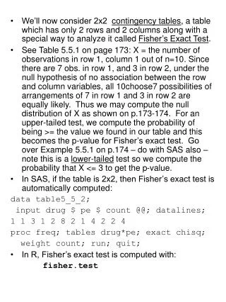
We’ll now consider 2x2 contingency tables, a table which has only 2 rows and 2 columns along with a special way to analyze it called Fisher’s Exact Test. • See Table 5.5.1 on page 173: X = the number of observations in row 1, column 1 out of n=10. Since there are 7 obs. in row 1, and 3 in row 2, under the null hypothesis of no association between the row and column variables, all 10choose7 possibilities of arrangements of 7 in row 1 and 3 in row 2 are equally likely. Thus we may compute the null distribution of X as shown on p.173-174. For an upper-tailed test, we compute the probability of being >= the value we found in our table and this becomes the p-value for Fisher’s exact test. Go over Example 5.5.1 on p.174 – do with SAS also – note this is a lower-tailed test so we compute the probability that X <= 3 to get the p-value. • In SAS, if the table is 2x2, then Fisher’s exact test is automatically computed: data table5_5_2; input drug $ pe $ count @@; datalines; 1 1 3 1 2 8 2 1 4 2 2 4 proc freq; tables drug*pe; exact chisq; weight count; run; quit; • In R, Fisher’s exact test is computed with: fisher.test
If you have paired data with dichotomous responses, then McNemar’s test is appropriate. The example given in Table 5.8.1 is a good one: to assess whether a debate changes a voter’s mind, we find out who a voter favors before and after the debate (paired). Table 5.8.1 shows the results... The hypothesis being tested is that the probability of switching from A to B is the same as the probability of switching from B to A. Let XAB = the number of switches from A to B and XBA = the number of switches from B to A. Under the null hypothesis of equal chance of switching from A to B as B to A, XAB is just like the sign test statistic with a B(n, .5) distribution. Standardize it and use Z or square the standardized statistic and use chi-square with 1 degree of freedom – this implementation is typically called McNemar’s test. • Apply this to the data in Table 5.8.1 – SAS implements McNemar’s test in PROC FREQ. R has mcnemar.test • HW: Read sections 5.5 (Fisher’s Exact Test) and 5.8 (McNemar’s Test). Do #7-9,12 and 13 at the end of Ch. 5. Begin reading in Chapter 8, Bootstrap Methods...