Download
1 / 22
220 likes | 237 Views
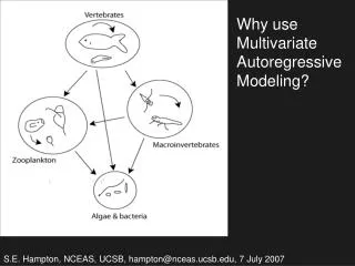
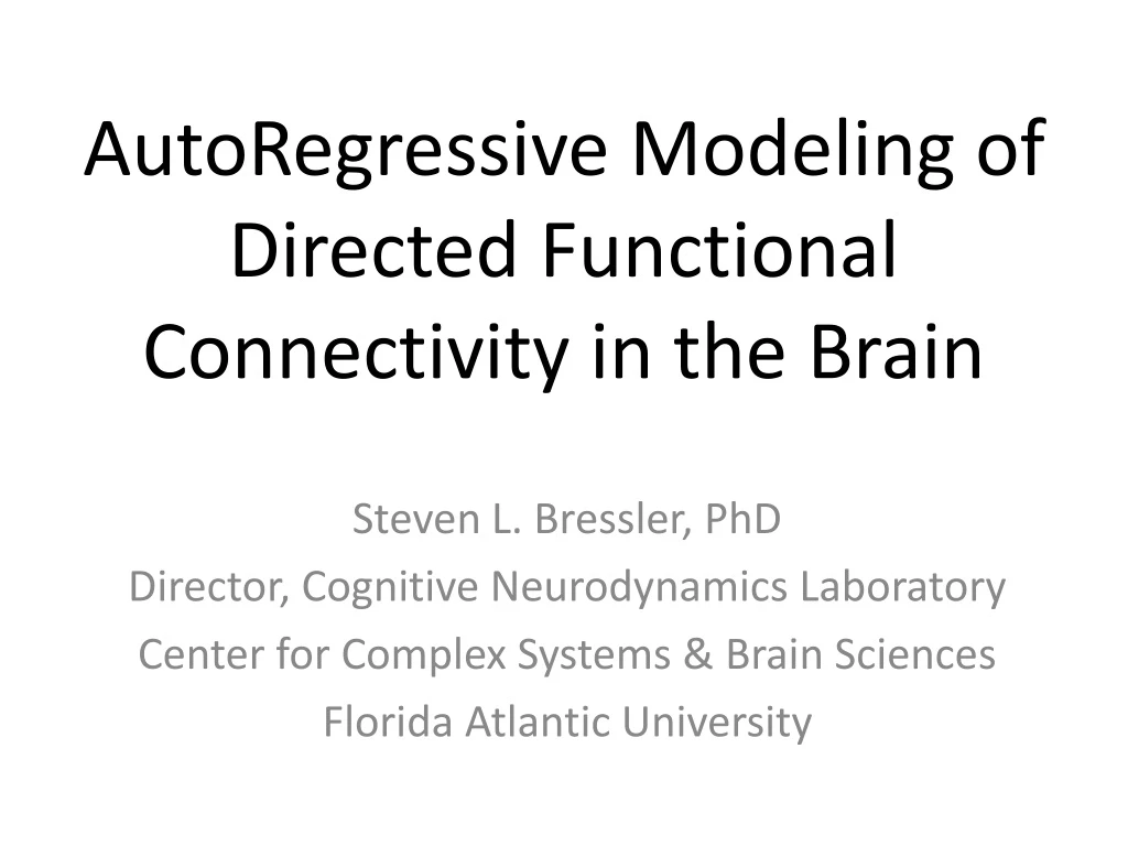
AutoRegressive Modeling of Directed Functional Connectivity in the Brain. Steven L. Bressler, PhD Director, Cognitive Neurodynamics Laboratory Center for Complex Systems & Brain Sciences Florida Atlantic University. Correlation. Causal Influence. Correlation vs Causal Influence.

E N D
AutoRegressive Modeling of Directed Functional Connectivity in the Brain Steven L. Bressler, PhD Director, Cognitive Neurodynamics Laboratory Center for Complex Systems & Brain Sciences Florida Atlantic University
Correlation CausalInfluence Correlation vs Causal Influence 2016 IOP World Congress Pre-Congress Course
Wiener Causality For two simultaneous time series, one series is called causal to the other if we can better predict the second series by incorporating knowledge of the first one. Norbert Wiener The Theory of Prediction, 1956 2016 IOP World Congress Pre-Congress Course
The AutoRegressive Model Xt= [a1Xt-1 + a2Xt-2 + a3Xt-3 + … + amXt-m] + εt where X is a zero-mean stationary stochastic process, ai are model coefficients, m is the model order, and εt is the white noise residual error process. 2016 IOP World Congress Pre-Congress Course
Wiener-Granger Causality Granger (1969): Let x1, x2, …, xt and y1, y2, …, yt represent two time series. Compare two linear autoregressive models: xt = a1xt-1 + … + amxt-m + t and xt = b1xt-1 + … + bmxt-m + c1yt-1 + … + cmyt-m + t If var(t) is significantly less than var(t), then the y time series significantly contributes to the x time series, and the y is said to have a casual influence on x. Restricted Model Unrestricted Model 2016 IOP World Congress Pre-Congress Course
Possible W-G Causality Relations Between Network Node Pairs • Unidirectional causality from x to y • Unidirectional causality from y to x • Bidirectional causality • Independence 2016 IOP World Congress Pre-Congress Course
Time-Domain Weiner-Granger Causality where Fyx is Weiner-Granger Causality, and Σ1 and Σ2 are the variances of t and t , respectively. 2016 IOP World Congress Pre-Congress Course
Frequency-Domain Weiner-Granger Causality Geweke (1982) found a frequency-domain (spectral) representation of W-G Causality, called Iyx(ω): SpectralW-G Causalityfrom y to x is: where ω is frequency in rads/sec,Sxx is the autospectrum of x,Hxx(ω) is an element of the transfer function H(ω)=A-1(ω), 2 is the residual variance of the unrestricted model of x, and * denotes complex conjugation and matrix transposition. 2016 IOP World Congress Pre-Congress Course
W-G Causality as Explained Power We see that spectral W-G Causality is defined based on the part of the total power of process x that is explained by process y. 2016 IOP World Congress Pre-Congress Course
Relation of Time-Domain & Frequency-Domain Weiner-Granger Causality W-G Causality from y to x in the time domain equals the sum of Spectral W-G Causalities from y to x over all frequencies. 2016 IOP World Congress Pre-Congress Course
Examples of W-G Spectra of Macaque Cortical Task-Related LFPs Indicating Beta-Frequency Unidirectional Causality 2016 IOP World Congress Pre-Congress Course
The MultiVariateAutoRegressive (MVAR) Model Xi,t= ai,1,1X1,t-1 + ai,1,2X1,t-2 + … + ai,1,mX1,t-m + ai,2,1X2,t-1 + ai,2,2X2,t-2 + … + ai,2,mX2,t-m + … + ai,p,1Xp,t-1 + ai,p,2Xp,t-2 + … + ai,p,m Xp,t-m + ei,t Xt = A1Xt-1 + + AmXt-m + Et where: Xt = [x1t , x2t , , xpt]T are p data channels, m is the model order,Ak are p x p coefficient matrices, & Et is the white noise residual error process vector. 2016 IOP World Congress Pre-Congress Course
MVAR Modeling of Event-Related LFP Time Series • LFP time series from repeated task trials are treated as realizations of a stationary stochastic process. • Ak are obtained by solving the multivariate Yule-Walker equations (of size mp2), using the Levinson, Wiggens, Robinson algorithm, as implemented by Morf et al. (1978). Morf M, Vieira A, Lee D, Kailath T (1978) Recursive multichannel maximum entropy spectral estimation. IEEE Trans Geoscience Electronics 16: 85-94) • The model order is determined by parametric testing. 2016 IOP World Congress Pre-Congress Course
W-G Causality Graphs • A set of network nodes may be analyzed for directed functional connectivity by computing W-G Causality in both directions between all node pairs. • The statistical significance of each W-G Causality is computed by comparison to a “permutation distribution”. • Significant W-G Causalities are plotted as arrows between nodes on a network graph, with arrow direction indicating the direction of W-G causal influence and arrow thickness representing the magnitude of W-G causal influence. 2016 IOP World Congress Pre-Congress Course
Example of a W-G Causality Graph from Macaque Cortical Task-Related LFPs(from Brovelli et al., PNAS, 2004) 2016 IOP World Congress Pre-Congress Course
Adaptive MultiVariateAutoRegressive (AMVAR) Modeling(Ding, Bressler et al., Biological Cybernetics, 2000) • AMVAR modeling captures the dynamics of AR processes with high temporal precision. • MVAR modeling is performed in a short time window, sliding with a high degree of overlap. • When spectral analysis is performed on the model at each time step, a time-frequency plot is obtained. 2016 IOP World Congress Pre-Congress Course
Example of AMVAR Time-Frequency Coherence Plot from Macaque Cortical Task-Related LFPs 2016 IOP World Congress Pre-Congress Course
Spectral Analysis by MVAR Modeling • The Spectral Matrix is defined as: S( f ) = <X (f ) X (f )*> = H(f ) H*(f ) where * denotes matrix transposition & complex conjugation; is the covariance matrix of Et ; and is the transfer function of the system. • The Power Spectrum of channel k is Skk( f ) which is the k th diagonal element of the spectral matrix. 2016 IOP World Congress Pre-Congress Course
Example of Power Spectrum of a Macaque Cortical Task-Related LFP Indicating Beta-Frequency Oscillatory Activity 2016 IOP World Congress Pre-Congress Course
Cross-Spectral Analysis by MVAR Modeling • The Cross-Spectrum of channels k & l is Skl( f ). • The (squared) Coherence Spectrum of channels k & l is the magnitude of the cross-spectrum normalized by the two auto-spectra: Ckl( f ) = |Skl( f )|2 / Skk( f ) Sll( f ). • The value of coherence at frequency f can range from 1, indicating maximum interdependence, down to 0, indicating no interdependence. The phase of the cross spectrum plotted as a function of f gives the phase spectrum. 2016 IOP World Congress Pre-Congress Course
Example of Coherence Spectrum of Macaque Cortical Task-Related LFPs Indicating Beta-Frequency Synchronization 2016 IOP World Congress Pre-Congress Course
Take-Home Message • The study of Directed Functional Connectivity (DFC) is an important approach to understanding brain function. • DFC can effectively be computed from neural data by AutoRegressive (AR) modeling. • AR modeling is especially useful for revealing the spectral profile of DFC in the brain on a short timescale. • Spectral analysis of neural data by AR modeling also reveals short-time brain network dynamics and graph properties. 2016 IOP World Congress Pre-Congress Course