Download
1 / 40
410 likes | 566 Views
A numerical method for barotropic flow simulation with applications to cavitation. M.V Salvetti, F. Beux, M. Bilanceri ( University of Pisa ) E. Sinibaldi (now at Scuola Superiore Sant’Anna, Pisa ). Micro-Macro Modelling and Simulation of Liquid-Vapour Flows Strasbourg, 23-25 January 2008.

E N D
A numerical method for barotropic flow simulation with applications to cavitation M.V Salvetti, F. Beux, M. Bilanceri (University of Pisa) E. Sinibaldi (now at Scuola Superiore Sant’Anna, Pisa) Micro-Macro Modelling and Simulation of Liquid-Vapour FlowsStrasbourg, 23-25 January 2008
Industrial and engineering motivation Development of a numerical tool for the prediction of the performance of axial inducers typical of turbopumps for liquid propellent rockets. rotating inducer non rotating cylindrical case The main role of the inducer is to increase the fluid pressure (velocity decrease) through rotation. Fundings from the Italian Space Agency and European Space Agency.
INFLOW Difficulties • Complex rotating 3D geometry. • Severe size limitations which lead to very high rotational speed cavitation phenomena need of a model to take into account cavitation. Choice of the cavitation model Considering the characteristics of the considered engineering problem (interest in global performance predictions, short life-time, cryogenic propellers, distribution of the active cavitation nuclei not known) Homogeneous-flow model, i.e. liquid/vapour mixture modeled as a single-phase fluid
Cavitation model Model proposed by L. d’Agostino et al. (2001), which takes into account (at least approximately) for thermal cavitation effects . Barotropic flow: the state equation relates pressure and density. In particular, for the considered model the state equation has the following form: liquid characteristic fluid physical parameters (known) liquid-vapour mixture Starting from this context, the more general scope of the research activity is to develop a numerical tool for the simulation of barotropic flows in complex geometry.
Cavitating flow behavior Difficulty: in the homogenous-flow description, the physical properties of the flow change dramatically between the zones of pure liquid and the cavitating regions (fluid/vapour mixture). speed of sound high speed of sound (H2O ~ 1400 m/s) M<<1 incompressible regime density high M supersonic-hypersonic flow
Modellazione dei flussi cavitanti • Flows characterized by nearly incompressible zones together with highly supersonic flow regions. two possible choices: Numerical solvers for incompressible flows suitably corrected to take into account compressibility Numerical discretization of the compressible flow equations unknown, p from the state equation p unknown Examples of applications to cavitating flows: van der Heul et al., ECCOMAS 2000, Senocack and Shyy, JCP 2002, …
Mathematical model Because of the barotropic state law the energy equation is decoupled only mass and momentum balances are considered • Equations for 3D laminar viscous compressible flows (no turbulence) in conservative variables or • Equations for 3D inviscid compressible flows in conservative variables + barotropic state equation (ODE or analytic laws)
Numerical discretization: outline • 1D inviscid flows • Spatial discretization of 1st order of accuracy (preconditioning) • Linearized implicit time advancing • Extension to 2nd order of accuracy in space (MUSCL) • Time advancing for 2nd order scheme (defect correction) • 3D inviscid flows (in rotating frames) • extension of the previous ingredients to tetrahedral unstructured grids • 3D laminar viscous flows • P1 finite-element discretization of viscous flows (not shown)
i-1,i i,i+1 Wi-1 Wi Wi+1 x Ci-1 Ci Ci+1 Numerical fluxes 1D inviscid flows:spatial discretization Galerkin projection on the finite-volume basis functions (piecewise constant) time discretization
Numerical fluxes Godunov-type flux: the exact solution of the Riemann problem between two neighboring cells is used. In the present research activity, a procedure has been developed for the construction of the Riemann problem solution for Euler equations and a generic convex barotropic law. Reference: E. Sinibaldi, Implicit preconditioned numerical schemes for the simulation of three-dimensional barotropic flows, Pisa, Edizioni della Normale, in press, ISBN 978-88-7642-310-9. • Exact 1D benchmark for generic barotropic state laws • Construction of a Godunov-type scheme
Numerical fluxes Roe scheme: approximated solution of the Riemann problem between two neighboring cells is used.. centered part upwind part Roe matrix numerical viscosity Contribution of the present research activity definition of the Roe matrix for a generic barotropic state law(PhD. Thesis by E. Sinibaldi or Sinibaldi, Beux & Salvetti, INRIA RR4891, 2003 (available on line), Sinibaldi, Beux & Salvetti, Flow Turbulence and Combustion 76(4), 2006).
Preconditioning for low-Mach numbers Problem: the numerical solvers for compressible flows suffer in general of accuracy problems if applied to low Mach flows. Following Guillard and Viozat (1999), an asymptotic analysis for M0 (Sinibaldi, Beux & Salvetti, 2003 or P.H.D. Thesis by E. Sinibaldi) shows that: • the continous solution is characterized by pressure variations in space of the order of M2 • the semi-discrete solution is characterized by pressure variations in space of the order of M preconditioning (following Guillard and Viozat, 1999) • the scheme becomes accurate also for M0 (asymptotic analysis) • preconditioning is applied only to the upwind part time consistency for unsteady problems The preconditioning matrix P is of Turkel-type (for its expression see Sinibaldi, Beux & Salvetti, Flow Turb. Comb. 2006 or P.H.D. Thesis by E. Sinibaldi).
Time discretization for 1st order schemes Adopted approach: implicit linearized scheme • Backward Euler implicit scheme: • We have shown that for the Roe scheme(Sinibaldi et al., 2003 and Sinibaldi P.h.D. Thesis): • Thus the implicit scheme can be linearized as follows: linear system (tridiagonal in 1D) NB: remark that we did not use the homogeneity of the Eulerian fluxes, which does not hold for generic barotropic state laws.
Space discretization:extension to 2nd order of accuracy Wi-1 Wi Wi+1 Adopted approach: MUSCL reconstruction Wijand Wjiare the extrapolated values of the variables at the cell interface Gradients can be computed in different ways, by combining different approximations (limited stencil + ad hoc coefficients) Wi-1,i Wi,i-1 • different schemes • 2nd order accurate • introducing a numerical viscosity proportional to 2th, 4th or 6th order derivatives (Camarri et al., Comp. Fluids 2004).
Time advancing for the 2nd order accurate scheme Adopted approach: defect correction • implicit formulation with a BDF method of order q: p-accurate discretization of the spatial differential operator • simpler non linear systems are iteratively considered (for p=2): second-order First-order • s-th DeC iteration after linearization: first-order linearized operator block tridiagonal linear system
Time advancing for the 2nd order accurate scheme Adopted approach: defect correction Full convergence of the DeC iteration is not needed to reach the higher order of accuracyin space and time (Martin and Guillard, Comput. & Fluids, 1996) • We have shown that, in our case, one DeC iteration is sufficient to reach 2-order (space and time) accuracy: block tridiagonal linear system: • For comparison, the fully 2-order linearized approach gives a block pentadiagonal system in 1D
Extension to 2D-3D Unstructured grids (tetrahedra) • Easy to build and to refine for 3D complex geometry With respect to structured grids: • Larger complexity of implementation of numerical algorithms • Larger computational requirements for fixed number of nodes.
Extension to 2D-3D (methodology developed at INRIA Sophia-Antipolis) nodes in the neighbourhood of node i Finite-volume dual grid (cells) obtained by using the medians of the tetrahedra faces normal integrated on the cell boundary Roe flux 1st order 2nd order
Rotating frames Extension to non-inertial frames rotating with a constant rotational speed • Incorporation of the non-inertial terms (Coriolis and centrifugal effects) in a source term (S) in the momentum equation. • Finite–volume discretization in space of S: with source term at node i • Linearized implicit time-discretization (to be incorporated in the scheme) through the Jacobian: diagonal term in linear system matrix known (RHS term) independent of time
Quasi-1D water flow in a nozzle STEADY-STATE IN a C-D SYMMETRICAL NOZZLE: cross-sectional area 1 2 source numerical transient Symmetrical grid, 360 cells, minimum spacing 0.02 (throat) 5.7 5.0 IN OUT Inlet B.C’s: Outlet B.C’s: I.C’s: Water in standard condition M 10-3 1st order of accuracy in space and Roe numerical flux
Quasi-1D water flow in a nozzle Effects of preconditioning on the solution accuracy Pressure distribution along the nozzle axis in non-cavitating conditions (pure liquid) non preconditioned • Preconditioning is actually important and works well in improving the numerical solution accuracy.
Quasi-1D water flow in a nozzle Effects of preconditioning and of the time advancing scheme on the numerical efficiency • For explicit time advancing, preconditiong significantly decreases the maximum allowable time step. This reduction becomes more important as the Mach number decreases prec=O(M)*noprec (see E. Sinibaldi PhD. Thesis) • The preconditioned linearized implicit scheme has practically no time steplimitation in non cavitating conditions. • In cavitating conditions, some improvements with respect to the explicit scheme are found, but severe limitations on the time-step remain.
Riemann problems • 1D numerical experiments for Riemann problems characterized by: • different barotropic laws (including the one for cavitating flows) • different characteristic waves • different regimes (low Mach, transonic) • Roe and Godunov fluxes (1st order of accuracy) • implicit linearized scheme • No differences between the results obtained with the Godunov scheme and with the Roe one the Godunov scheme will not be used in other applications (2D, 3D) because much more computationally demanding • For non-cavitating barotropic laws the results show: • accuracy consistent with the used 1st order accurate approximation, • satisfactory efficiency of time advancing.
Riemann problems • flow regime: low Mach • flow regime: generic Mach • barotropic law: • barotropic law: • 2 shocks • shock and rarefaction p 600 cells 4000 cells u u stationary contact blow-up for c(CFL) 10 blow-up for c(CFL) 100
Riemann problem for the cavitation barotropic law • flow regime: low Mach / high Mach 4000 cells • barotropic law: LdA model for cavitation 2 rarefactions head p u pressure tail pressure (detail) p’ p barotropic curve, for reference tail !!! ’
Riemann problem for the cavitation barotropic law head p pressure, for reference density tail p’ density (detail) barotropic curve, for reference ’ • Very fine spatial discretization and small time steps are needed to capture pressure and density “spikes” in the cavitating region 4000 cells
IN OUT Water flow around a hydrofoil mounted in a tunnel (Beux et al.,M2AN, 2005) Dirichlet homog. Neumann • Inviscid flow. • 1st order of accuracy and Roe scheme • Linearized implicit time advancing Free-streams(T = 293.16 K): cavitation number non-cavitating cavitating Grids: GR1 (det.) GR2 cells tetrahedra
almost independent of the grid effect of = 0.1 = 0.01 Water flow around a hydrofoil mounted in a tunnel (Beux et al.,M2AN, 2005) test-section Pressure distribution over the hydrofoil Centro Spazio, Pisa local preconditioning only in the cavitating region • Surprisingly good accuracy. • Problems of efficiency: non-cavitating simulations CFL up to 400, with cavitation CFLmax = 10-2
Water flow around a hydrofoil mounted in a tunnel (Beux et al.,M2AN, 2005) local cavitation number Mach sigma Mach up to 28 = 0.1 less pronounced Mach variation, OK more extended cavity, OK Mach up to 11 = 0.01
Some Remarks • First series of test-cases (inviscid flows, 1st order of accuracy in space, preconditioning, linearized implicit time advancing): • quasi-1D water flow in a nozzle (non cavitating and cavitating conditions) • Riemann problems with different barotropic state laws • water flow around a hydrofoil (non cavitating and cavitating conditions) • water flow in a turbopump inducer in non-cavitating conditions (not shown) • Satisfactory accuracy (in the limit of the assumptions made) in both non-cavitating and cavitating conditions. • Numerical efficiency problems when cavitating regions are present. • Additional series of 1D numerical experiments: • to investigate whether the efficiency problems in cavitating conditions are due to the adopted linearization technique for time advancing • to test the efficiency of the defect correction approach for 2nd order accuracy simulations in non-cavitating conditions
Additional series of 1D numerical experiments: linearized implicit vs. fully non-linear implicit in cavitating conditions Test-case: Riemann problem • 2 initial liquid states 2 rarefactions • LdA cavitating flow state equation Solution accuracy Pressure field at t=1s Discretization: 4000 cells -100 -2000 2000 100 detail Robustness and computational cost • No improvement in robustness with the fully implicit formulation as for non cavitating flows, the fully implicit simulations blow up at lower CFL than the ones with the linearized implicit scheme. • For the same resolution in space and the same time step, the computational costs are much larger for the fully implicit scheme.
Validation of 2-order formulation: 1D numerical experiments TEST-CASE 1: Quasi-1D water flow in a convergent-divergent nozzle • flow regime: steady and supersonic • barotropic law: FO Density field Spatial discretization: 400 cells Comparison of implicit formulations FO: first-order (in space and time) linearized implicit slope 1 2-order (in space and time) linearized implicit DeCDefect correction approach DeC with 1 and 2 inner iterations SO: fully second-order linearized implicit FU:fully implicit second-order(non linear solver (PETSc library) based on a gradient-free Newton-GMRES approach) Velocity error log-log scale slope 2
TEST-CASE 2: Riemann problem (shock and rarefaction) • flow regime: unsteady and subsonic barotropic law: velocity field (t=1 s) Spatial refinement Temporal discretization: t=0.0001 40 cells 400 cells temporal refinement Spatial discretization: 400 cells DeC2, DeC3 DeC1 t=0.01 t=0.001
Additional series of 1D numerical experiments: Validation of the second-order formulation Solution accuracy • No loss of accuracy with the present formulation: • neither due to the defect correction comparison DeC/fully second-order linearized implicit • nor due to the linearization of the implicit time-advancing comparison linearized implicit/fully implicit formulations • In accordance with the theoretical appraisal, one iteration of defect correction is already sufficient to reach 2nd order accuracy • Nevertheless, for particular cases (large CFL number), a second inner iteration can improve the solution (stabilization effect) Computational cost • Steady regimes: the steady solution is obtained after very few pseudo-time iterations for all the linearized implicit approaches while the fully implicit formulation needs a CFL-like condition (for fine spatial discretization, i.e. large dimension of the non linear system)). • For the same grid and time step, DeC1 is approximately two times cheaper than the fully second-order linearized implicit approach. A larger ratio is expected for 3D cases due to the increase of complexity and stiffness.
Concluding Remarks and Developments • For non-cavitating barotropic flows, the proposed numerical methodology shows satisfactory: • accuracy (MUSCL reconstruction + preconditioning for low Mach) • robustness and efficiency (linearized implicit time advancing + defect correction) • For cavitating flows and the homogeneous flow model: • severe restriction of the time step are observed unaffordable CPU requirements for 3D simulations • numerical experiments show that this is not due to the adpted linearization of the implicit time advancing • For cavitating flows described through the homogenous-flow model: • try more robust numerical fluxes (HLL, HLLC) and/or • relaxion techniques in time • Change cavitation model (two-phases) Application of the numerical set-up (as it is) to the simulation of problems characterized by barotropic laws less stiff than the cavitating one (shallow water, atmosphere…)
Cavitating flow behavior pressure liquid: ~ incompressible liquid-vapour mixture: highly compressible density
Time advancing for the 2nd order accurate scheme Full second-order linearized approach
inducer nose afterbody Flusso di acqua in un induttore di turbopompa (Sinibaldi et al., 2006) inter-blade covering: no gap very complex geomety (detail of hub-blade intersection) Free-stream(T = 296.16 K): 2.5x10⁶ elements
Flusso di acqua in un induttore di turbopompa (Sinibaldi et al., 2006) pressure contours velocity (longitudinal cut plane) max (red) 177700 [Pa] min (blue) 79700 [Pa] spacing 5000 [Pa] axial back-flow correctly described! pretty nice results… it seems a promising scheme! (cavitating simulation not affordable -at a “reasonable” cost- due to the efficiency issue)
since free model parameter Homogeneous-flow modelsThermal barotropic model (d’Agostino et al., 2001) pure liquid:weakly compressible fluid mixture In which L, g*, pc, V are constants dependent on the considered flow