Download
1 / 67
680 likes | 807 Views
Lecture 2 Probability and what it has to do with data analysis. Abstraction. Random variable, x it has no set value, until you ‘realize’ it its properties are described by a probability, P. One way to think about it. pot of an infinite number of x’s. x. p(x).

E N D
Lecture 2 Probability and what it has to do with data analysis
Abstraction Random variable, x it has no set value, until you ‘realize’ it its properties are described by a probability, P
One way to think about it pot of an infinite number of x’s x p(x) Drawing one x from the pot “realizes” x
Describing P If x can take on only discrete values, say (1, 2, 3, 4, or 5) then a table would work: 40% probability that x=4 Probabilities should sum to 100%
Probability should sum to 1 Sometimes you see probabilities written as fractions, instead of percentages 0.15 probability that x=4 And sometimes you see probabilities plotted as a histogram 0.5 0.15 probability that x=4 P(x) 0.0 x 1 2 3 4 5
probability that x is between x1 and x2 is proportional to this area If x can take on any value, then use a smooth function (or “distribution”) p(x) instead of a table p(x) x x1 x2 mathematically P(x1<x<x2) = x1x2p(x) dx
p(x) x Probability that x is between - and + is 100%, so total area = 1 Mathematically -+p(x) dx = 1
One Reason Why all this is relevant … Any measurement of data that contains noise is treated as a random variable, d and …
The distribution p(d) embodies both the ‘true value’ of the datum being measured and the measurement noise and …
All quantities derived from a random variable are themselves random variables, so …
The algebra of random variables allows you to understand how … … measurement noise affects inferences made from the data
Basic Description of Distributionswant two basic numbers1) something that describes what x’s commonly occur2) something that describes the variability of the x’s
1) something that describes what x’s e commonly occurthat is, where the distribution is centered
Mode x at which distribution has peak most-likely value of x peak p(x) x xmode
The most popular car in the US is the Honda CR-V Honda CV-R But the next car you see on the highway will probably not be a Honda CR-V Where’s a CV-R?
But modes can be deceptive … 100 realizations of x x N 0-1 3 1-2 18 2-3 11 3-4 8 4-5 11 5-6 14 6-7 8 7-8 7 8-9 11 9-10 9 Sure, the 1-2 range has the most counts, but most of the measurements are bigger than 2! peak p(x) x 0 10 xmode
Median 50% chance x is smaller than xmedian 50% chance x is bigger than xmedian No special reason the median needs to coincide with the peak p(x) 50% 50% x xmedian
Expected value or ‘mean’ value you would get if you took the mean of lots of realizations of x Let’s examine a discrete distribution, for simplicity ... 4 3 P(x) 2 1 0 1 2 3 x
Hypothetical table of 140 realizations of x x N • 20 • 80 • 40 Total 140 mean = [ 20 1 + 80 2 + 40 3 ] / 140 = (20/140) 1+ (80/140) 2 + (40/140) 3 = p(1) 1+ p(2) 2 + p(3) 3 = Σi p(xi) xi
by analogyfor a smooth distribution Expected (or mean) value of x E(x) = -+x p(x) dx
2) something that describes the variability of the x’sthat is, the width of the distribution
Here’s a perfectly sensible way to define the width of a distribution… p(x) 50% 25% 25% x W50 … it’s not used much, though
Width of a distribution Here’s another way… Parabola [x-E(x)]2 p(x) x E(x) … multiply and integrate
Idea is that if distribution is narrow, then most of the probability lines up with the low spot of the parabola [x-E(x)]2 p(x) x E(x) But if it is wide, then some of the probability lines up with the high parts of the parabola [x-E(x)]2p(x) Compute this total area … x E(x) Variance = s2= -+[x-E(x)]2p(x) dx
variance = s A measure of width … p(x) s x E(x) we don’t immediately know its relationship to area, though …
the Gaussian or normal distributionp(x) = exp{ - (x-x)2 / 2s2 ) s2is variance x is expected value 1 (2p)s Memorize me !
p(x) x = 1 s= 1 Examples of Normal Distributions x p(x) x = 3 s= 0.5 x
x x+2s x-2s Properties of the normal distribution Expectation = Median = Mode = x 95% of probability within 2sof the expected value p(x) 95% x
Again, Why all this is relevant … Inference depends on data … You use measurement, d, to deduce the values of some underlying parameter of interest, m. e.g. use measurements of travel time, d, to deduce the seismic velocity, m, of the earth
model parameter, m, depends on measurement, d so m is a function of d, m(d) so …
If data, d, is a random variable then so is model parameter, m All inferences made from uncertain data are themselves uncertain Model parameters are described by a distribution, p(m)
Functions of a random variable any function of a random variable is itself a random variable
Special case of a linear relationship and a normal distribution Normal p(d) with mean d and variance s2d Linear relationship m = a d + b Normal p(m) with mean ad+b and variance a2s2d
Example Liberty island is inhabited by both pigeons and seagulls 40% of the birds are pigeons and 60% of the birds are gulls 50% of pigeons are white and 50% are grey 100% of gulls are white
Two variables species s takes two values pigeon p and gull g color c takes two values white w and tan t Of 100 birds, 20 are white pigeons 20 are grey pigeons 60 are white gulls 0 are grey gulls
What is the probability that a bird has species s and color c ? a random bird, that is p 20% 20% s g 60% 0% Note: sum of all boxes is 100% w t c
Two continuous variablessay x1 and x2have a joint probability distributionand writtenp(x1, x2)with p(x1, x2) dx1 dx2 = 1
You would contour a joint probability distributionand it would look something like x2 x1
What is the probability that a bird has color c ? Of 100 birds, 20 are white pigeons 20 are grey pigeons 60 are white gulls 0 are grey gulls start with P(s,c) p 20% 20% s g 60% 0% w t and sum columns c To get P(c) 80% 20%
What is the probability that a bird has species s ? start with P(s,c) p 20% 20% 40% and sum rows s Of 100 birds, 20 are white pigeons 20 are grey pigeons 60 are white gulls 0 are grey gulls g 60% 0% 60% w t To get P(s) c
These operations make sense with distributions, too x2 x2 x2 x1 x1 p(x2) p(x1) x1 p(x1) = p(x1,x2) dx2 p(x2) = p(x1,x2) dx1 distribution of x1 (irrespective of x2) distribution of x2 (irrespective of x1)
p 50% 50% s g 100% 0% w t c Given that a bird is species swhat is the probability that it has color c ? Of 100 birds, 20 are white pigeons 20 are grey pigeons 60 are white gulls 0 are grey gulls Note, all rows sum to 100
This is called theConditional Probability of c given sand is writtenP(c|s)similarly …
Given that a bird is color cwhat is the probability that it has species s ? Of 100 birds, 20 are white pigeons 20 are grey pigeons 60 are white gulls 0 are grey gulls So 25% of white birds are pigeons p 25% 100% s g 75% 0% w t Note, all columns sum to 100 c
This is called theConditional Probability of s given cand is writtenP(s|c)
Beware!P(c|s) P(s|c) p p 50% 50% 25% 100% s s g 100% 0% g 75% 0% w t w t c c
Actor Patrick Swaysepancreatic cancer victim Lot of errors occur from confusing the two: Probability that, if you have pancreatic cancer, that you will die from it 90% Probability that, if you die, you will have died of pancreatic cancer 1.4%
p 25 100 p 20 20 s s g 75 0 g 60 0 w t c w t 80 20 c note P(s,c) = P(s|c) P(c) 25% of 80 is 20 = w t c