Download
1 / 14
140 likes | 299 Views
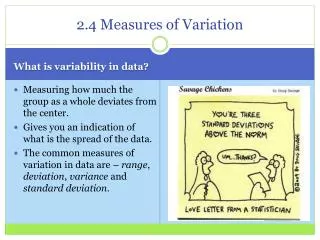
2.4 Measures of Variation. What is variability in data?. Measuring how much the group as a whole deviates from the center. Gives you an indication of what is the spread of the data. The common measures of variation in data are – range , deviation , variance and standard deviation.

E N D
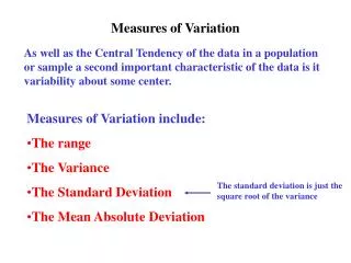
2.4 Measures of Variation What is variability in data? • Measuring how much the group as a whole deviates from the center. • Gives you an indication of what is the spread of the data. • The common measures of variation in data are – range, deviation, variance and standard deviation.
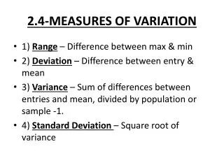
Range The range is the simplest measure of variation. It is difference between the biggest and smallest random variable. Range = Maximum value - Minimum value Range has the advantage of being easy to compute. Its disadvantage, however, is that it uses only two entries from the entire data set. Age based on class survey data: 26, 25, 35, 35, 40, 41, 21, 19, 20, 20, 30, 25, 24, 47, 36, 16, 23, 48, 40, 21, 27, 22, 39, 34, 26, 25, 16, 24, 33, 32, 28, 48, 40, 38. Range = maximum – minimum = 48 – 16 = 32
Deviation, Variance and Standard Deviation The deviation of an entry xiin a data set is the difference between that entry and the mean μ of the data set i.e. xi– μ The populationvariance of the population data set of N entries is: The population standard deviation is the square root of the population variance i.e. The samplevariance of the sample data set of N entries is: The sample standard deviation is the square root of the sample variance i.e.
Deviation, Variance and Standard Deviation Age based on class survey: 26, 25, 35, 35, 40, 41, 21, 19, 20, 20, 30, 25, 24, 47, 36, 16, 23, 48, 40, 21, 27, 22, 39, 34, 26, 25, 16, 24, 33, 32, 28, 48, 40, 38. Population size N = 34, Population mean μ = 1024/34 = 30.11765 σ2 = 82.2803 σ = 9.0708
Deviation, Variance and Standard Deviation Variance and standard deviation take into consideration all the data. However they are both easily influenced by extreme scores since it is a square term. Variance is hard to interpret since it is a squared measure, standard deviation is interpreted as the average deviation from the mean.
Interpreting Standard Deviation When interpreting the standard deviation, remember that it is a measure of the typical amount an entry deviates from the mean. The more the entries are spread out, the greater the standard deviation.
Interpreting Standard Deviation Empirical Rule or The 68-95-99.7 rule: For a bell shaped symmetric distribution 68% of the data lies within one standard deviation of the mean, 95% of the data lies within two standard deviations of the mean and 99.7% of the data lies within 3 standard deviations of the mean.
Interpreting Standard Deviation Chebychev’s theorem When the distribution is not bell shaped or symmetric then this theorem gives a lower bound to the proportion of data the lies with k standard deviations of the mean. It states that: The proportion of any data set lying within k standard deviations of the mean is at least • k=2, In any data set, at least i.e. 75% of the data lies within 2 standard deviations of the mean.
Standard Deviation of Grouped Data Sample standard deviation for a frequency distribution is: Where c is the number of classes, xi is the ith data point in the sample, fi is the corresponding frequency, n is the sample size.
2.5 Measures of Position What are measures of position? • A measure of position gives you some idea of where particular data values would rank in an ordering of a data set • where a data value falls with respect to the mean of the sample or population..
Quartiles Quartiles divide the data into 4 equal parts. We need three quartiles to divide any data set into 4 equal parts, Q1, Q2and Q3. • About a quarter of the data falls below the first quartile, Q1 • About a half of the data falls below the second quartile, Q2 • About three quarters of the data falls below the third quartile, Q3 Interquartile range (IQR) of a data set is the difference between the third and first quartiles, Q3– Q1
Quartiles In essence five values can use used to describe a data set: Minimum data value, three quartiles - Q1, Q2, Q3 and maximum data value. These five numbers are called the five number summary since they describe the central tendency, the spread and the variation in the data. Drawing a Box-whisker plot • Find the five-number summary of the data set. • Construct a horizontal; scale that spans the range of the data. • Plot the five number above the horizontal scale. • Draw a box above the horizontal scale from Q1to Q3 and draw a vertical line in the box at Q2. • Draw whiskers from the box to minimum and maximum entries For the age data: Min = 16, Q1=23.25, Q2 = 27.5, Q3 = 37.5, Max = 48 Whisker Box Whisker Min entry Q1 Q2, Median Q3 Max entry
Percentiles and Other Fractiles Fractiles are numbers that divide an ordered data set into equal parts. Some commonly used fractiles are:
z-score The standard score or z-score, represents the number of standard deviations a given value x falls from the mean μ. To find the z-score for a given value, A z-score can be positive, negative or zero. If z is positive, the data point > the mean, If z is negative, the data point < the mean, If z = 0, the data point = mean.