Comprehensive Guide to Multiple Regression Analysis
Explore multiple regression model, interpreting coefficients, estimating expected values, model assessment, and predictions. Utilize regression analysis software for coefficient estimation.

Comprehensive Guide to Multiple Regression Analysis
E N D
Presentation Transcript
MultipleRegression Chapter 13
Introduction • In this chapter we extend simple linear regression where we had one explanatory variable, and allow for any number of explanatory variables. • We expect to build a model that fits the data better than the simple linear regression model.
Introduction • We shall use computer printout to • Assess the model • How well it fits the data • Is it useful • Are any required conditions violated? • Employ the model • Interpreting the coefficients • Predictions using the prediction equation • Estimating the expected value of the dependent variable
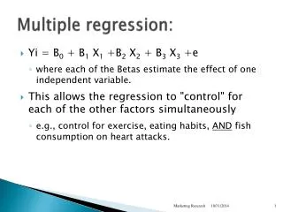
The Multiple Regression Model Idea: Examine the linear relationship between 1 response variable (y) & 2 or more explanatory variables (xi) Population model: Y-intercept Population slopes Random Error Estimated multiple regression model: Estimated (or predicted) value of y Estimated intercept Estimated slope coefficients
Simple Linear Regression y Observed Value of y for xi εi Slope = b1 Predicted Value of y for xi Random Error for this x value Intercept = b0 x xi
Y • * • * • * • * • * • * • * • * • * • * • * • * • * • * • * • * • X • * • 1 • X • 2 Multiple Regression, 2 explanatory variables • Least Squares Plane (instead of line) • Scatter of points around plane are random error.
Multiple Regression Model Two variable model y Sample observation yi < yi < e = (yi – yi) x2i x2 x1i < The best fit equation, y , is found by minimizing the sum of squared errors, e2 x1
Estimating the Coefficients and Assessing the Model • The procedure used to perform regression analysis: • Obtain the model coefficients and statistics using statistical software. • Diagnose violations of required conditions. Try to remedy problems when identified. • Assess the model fit using statistics obtained from the sample. • If the model assessment indicates good fit to the data, use it to interpret the coefficients and generate predictions.
Estimating the Coefficients and Assessing the Model, Example • Predicting final exam scores in BUS/ST 350 • We would like to predict final exam scores in 350. • Use information generated during the semester. • Predictors of the final exam score: • Exam 1 • Exam 2 • Exam 3 • Homework total
Estimating the Coefficients and Assessing the Model, Example • Data were collected from 203 randomly selected students from previous semesters • The following model is proposedfinal exam = b0 + b1exam1 + b2exam2 + b3exam3 + b4hwtot
Regression Analysis, Excel Output This is the sample regression equation (sometimes called the prediction equation) Final exam score = 0.0498 + 0.1002exam1 + 0.1541exam2 + 0.2960exam3 +0.1077hwtot
Interpreting the Coefficients • b0 = 0.0498. This is the intercept, the value of y when all the variables take the value zero. Since the data range of all the independent variables do not cover the value zero, do not interpret the intercept. • b1 = 0.1002. In this model, for each additional point on exam 1, the final exam score increases on average by 0.1002 (assuming the other variables are held constant).
Interpreting the Coefficients • b2 = 0.1541. In this model, for each additional point on exam 2, the final exam score increases on average by 0.1541 (assuming the other variables are held constant). • b3 = 0.2960. For each additional point on exam 3, the final exam score increases on average by 0.2960 (assuming the other variables are held constant). • b4 = 0.1077. For each additional point on the homework, the final exam score increases on average by 0.1077 (assuming the other variables are held constant).
Final Exam Scores, Predictions • Predict the average final exam score of a student with the following exam scores and homework score: • Exam 1 score 75, • Exam 2 score 79, • Exam 3 score 85, • Homework score 310 • Use trend function in Excel Final exam score = 0.0498 + 0.1002(75)+0.1541(79) + 0.2960(85) + 0.1077(310) = 78.2857
Model Assessment • The model is assessed using three tools: • The standard error of the residuals • The coefficient of determination • The F-test of the analysis of variance • The standard error of the residuals participates in building the other tools.
Standard Error of Residuals • The standard deviation of the residuals is estimated by the Standard Error of the Residuals: • The magnitude of seis judged by comparing it to
Regression Analysis, Excel Output Standard error of the residuals; sqrt(MSE) (standard error of the residuals)2: MSE=SSE/198 Sum of squares of residuals SSE
Standard Error of Residuals • From the printout, se = 11.5122…. • Calculating the mean value of y we have • It seems se is not particularly small. • Question:Can we conclude the model does not fit the data well?
Coefficient of Determination R2(like r2 in simple linear regression • The proportion of the variation in y that is explained by differences in the explanatory variables x1, x2, …, xk • R2 = 1 – (SSE/SSTotal) • From the printout, R2 = 0.382466… • 38.25% of the variation in final exam score is explained by differences in the exam1, exam2, exam3, and hwtot explanatory variables. 61.75% remains unexplained. • When adjusted for degrees of freedom, Adjusted R2 = 36.99%
Testing the Validity of the Model • We pose the question: Is there at least one explanatory variable linearly related to the response variable? • To answer the question we test the hypothesis H0: b1 = b2 = … = bk=0 H1: At least one bi is not equal to zero. • If at least one bi is not equal to zero, the model has some validity.
Testing the Validity of the Final Exam Scores Regression Model • The hypotheses are tested by what is called an F test shown in the Excel output below MSR/MSE P-value k = n–k–1 = n-1 = SSR MSR=SSR/k MSE=SSE/(n-k-1) SSE
Testing the Validity of the Final Exam Scores Regression Model [Variation in y] = SSR + SSE. Large F results from a large SSR. Then, much of the variation in y is explained by the regression model; the model is useful, and thus, the null hypothesis H0 should be rejected. Reject H0 when P-value < 0.05
Testing the Validity of the Final Exam Scores Regression Model Conclusion: There is sufficient evidence to reject the null hypothesis in favor of the alternative hypothesis. At least one of the bi is not equal to zero. Thus, at least one explanatory variable is linearly related to y. This linear regression model is valid The P-value (Significance F) < 0.05 Reject the null hypothesis.
Test statistic Testing the Coefficients • The hypothesis for each bi is • Excel printout H0: bi= 0 H1: bi¹ 0 d.f. = n - k -1

