A Predator-Prey Model

1. A Predator-Prey Model G. F. Fussmann, S. P. Ellner, K. W. Shertzer and G. Hairston Jr. (2000) Science, 290, 1358-1360

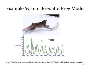
2. Background • Models for the interaction of prey and predators date back to the beginning of the 19th century (Volterra-Lotke equations) • In some conditions, both predator and prey populations oscillate. • The famous Canadian lynx data show this, for example.

3. The Experiment • A tank contains a species of algae, Chlorella vulgaris. • Nitrogen is the resource that limits algae growth, and this is controlled in the experiment. • The predator is a planktonic rotifer, Brachionis calyciflorus, that feeds on the algae.

4. Variables • N: Nitrogen concentration: prey nutrient • C: Prey concentration - Chlorella • R: Predator concentration - Reproducing Brachionus • B: Total Brachionus concentration

5. Predator-Prey differential equations

6. where the two F functions are thresholding functions that vary between zero and an upper asymptote:

7. Experimental Constants • bc = 3.30, bB = 2.25 • Kc = 4.3, KB = 15.0 • ε = 0.25 • M = 0.055 • λ = 0.400 • Ni = 80

8. Model parameter δ (dilution level) This parameter controls how rapidly the tank nitrogen level responds to a change in input nitrogen, and also how rapidly the prey population responds to this change.

9. At low dilution level δ, both predator and prey populations decay to zero. • At medium rates, the two populations are stable. • At higher rates, the two populations oscillate. • At even higher rates, the two populations again decay.

10. Fig. 1. Population dynamics predicted by the original model (left panels) and observed in the chemostat experiments (right panels).

12. What we would like to do • Use the data to estimate dilution rate δ, • compute the fit to the data based on the differential equation, • allow for some unexplained residual variation, • and deliver a reasonable confidence interval for δ.