Principal Component Analysis (PCA) for Clustering Gene Expression Data
340 likes | 558 Views
Principal Component Analysis (PCA) for Clustering Gene Expression Data. K. Y. Yeung and W. L. Ruzzo. Outline. Motivation of PCA and this paper Approach of this paper Data sets Clustering algorithms and similarity metrics Results and discussion. Why Are We Interested in PCA?.

Principal Component Analysis (PCA) for Clustering Gene Expression Data
E N D
Presentation Transcript
Principal Component Analysis(PCA) for ClusteringGene Expression Data K. Y. Yeung and W. L. Ruzzo
Outline • Motivation of PCA and this paper • Approach of this paper • Data sets • Clustering algorithms and similarity metrics • Results and discussion
Why Are We Interested in PCA? • PCA can reduce the dimensionality of the data set. • Few PCs may capture most of the variation in the original data set. • PCs are uncorrelated and ordered. • We expect the first few PCs may ‘extract’ the cluster structure in the original data set.
What Is This Paper for? • A theoretical result shows that the first few PCs may not contain cluster information. (Chang, 1983). • Chang’s example. • A motivating example. (Coming next).
A Motivating Example • Data: A subset of the sporulation data (477 genes) were classified into seven temporal patterns (Chu et al., 1998) • The first 2 PCs contains 85.9% of the variation in the data. (Figure 1a) • The first 3 PCs contains 93.2% of the variation in the data. (Figure 1b)
Sporulation Data • The patterns overlap around the origin in (1a). • The patterns are much more separated in (1b).
The Goal • EMPIRICALLY investigate the effectiveness of clustering gene expression data using PCs instead of the original variables.
The Setting • Genes are to be clustered, and the experimental conditions are the variables. • Assume there is an objective external criterion to cluster the data. The quality of clustering is measured by its distance to this gold standard here. • Assume the number of clusters is known.
Agreement Between Two Partitions The Rand index (Rand, 1971): Given a set of n objects S, let U and V be two different partitions of S. Let: a = # of pairs that are placed in the same cluster in U and in the same cluster in V d = # of pairs that are placed in different clusters in U and in different clusters in V Rand index = (a+d)/
Agreement (Cont’d) The adjusted Rand index (ARI, Hubert & Arabie, 1985): Note: Higher ARI means higher correspondence between two partitions.
Subset of PCs • Motivated by Chang’s example, it is possible to find other subsets of PCs to preserve the cluster structure better than the first few PCs. • How? --- The greedy approach. --- The modified greedy approach.
The Greedy Approach Let m0 be the minimum number of PCs to be clustered, and p be the number of variables in the data. • Search for a set of m0 PCs with maximum ARI, denoted as sm0. • For each m=(m0+1),…p, add another PC to s(m-1) and calculate ARI. The PC giving the maximum ARI is then added to get sm.
The Modified Greedy Approach • In each step of the greedy approach (# of PCs = m), retain the k best subsets of PCs for the next step (# of PCs = m+1). • If k=1, this is just the greedy approach. • k=3 in this paper.
The Scheme of the Study Given a gene expression data set with n genes (subjects) and p experimental conditions (variables), apply a clustering algorithm to • the given data set. • the first m PCs where m=m0,…p. • the subset of PCs found by the (modified) greedy approach. • 30 sets of random PCs. • 30 sets of random orthogonal projections.
Data Sets • “Class” refers to a group in the gold standard. “Cluster” refers to clusters obtained by a clustering algorithm. • There are two real data sets and three synthetic data sets in this study.
The Ovary Data • The data contains 235 clones and 24 tissue samples. • For the 24 tissue samples, 7 are from normal tissues, 4 from blood samples, and 13 from ovarian cancers. • The 235 clones were found to correspond four different genes (classes), each having 58, 88, 57 and 32 clones. • The data for each clone was normalized across the 24 experiments to have mean 0 and variance 1.
The Yeast Cell Cycle Data • The data set shows the fluctuation of expression levels over two cell cycles. • 380 gene were classified into five phases (classes). • The data for each gene was normalized to have mean 0 and variance 1 across each cell cycle.
Mixture of Normal on Ovary • In each gene (class), the sample covariance matrix and the mean vector are computed. • Sample (58, 88, 57, 32) clones from the MVN in each class. 10 replicates. • It preserves the mean and covariance of the original data, but relies on the MVN assumption.
Randomly Resample Ovary Data • For each class c (c=1,…,4) under experimental condition j (j=1,…,24), resample the expression level with replacement. Retain the size of each class. 10 replicates. • No MVN assumption. The independent sampling for different experimental conditions is reasonable as inspected.
Cyclic Data • This data set models cyclic behavior of genes over different time points. • It uses sin function and normal random numbers. • A drawback of this model is the arbitrary choice of several parameters.
Clustering Algorithmsand Similarity Metrics Clustering algorithms: • Cluster affinity search technique (CAST) • Hierarchical average-link algorithm • K-mean algorithm Similarity metrics: • Euclidean distance (m0=2) • Correlation coefficient (m0=3)
Table 2 • One sided Wilcoxon signed rank test. • CAST always favorites ‘no PCA’. • The two significances for PCA are not clear sucesses.
Conclusion • The quality of clustering results on the data after PCA is not necessarily higher than that on the original data, sometimes lower. • The first m PCs do not give the highest adjusted Rand index, i.E. Another set of PCs gives higher ARI.
Conclusion (Cont’d) • There are no clear trends regarding the choice of optimal number of PCs over all the data sets and over all the clustering algorithms and over the different similarity metrics. There is no obvious relationship between cluster quality and the number or set of PCs used.
Conclusion (Cont’d) • On average, the quality of clusters obtained by clustering random sets of PCs tend to be slightly lower than those obtained by clustering random sets of orthogonal projections, esp. when the number of components is small.
Grand Conclusion In general, we recommend AGAINST using PCA to reduce dimensionality of the data before applying clustering algorithms unless external information is available.