Technical Note 2. Linear Programming
Technical Note 2. Linear Programming. Optimizing the Use of Resources with Linear Programming (LP) LP is used in problems where resources are constrained or limited and certain assumptions are met Usually there is one objective (function)

Technical Note 2. Linear Programming
E N D
Presentation Transcript
Technical Note 2. Linear Programming • Optimizing the Use of Resources with Linear Programming (LP) • LP is used in problems where resources are constrained or limited and certain assumptions are met • Usually there is oneobjective (function) • Maximize profit, minimize cost, minimize distance traveled, etc. • Goal programming approach allows for multiple objectives • Some application areas:Aggregate sales and operations planningService/manufacturing productivity analysisProduct planningProduct routing Vehicle/crew schedulingDetermining optimal production and shipment (destination) routes
Linear Programming Assumptions • Linearity is a requirement of the model in both objective function and constraints • Homogeneity of products produced (i.e., products must the identical) and all hours of labor used are assumed equally productive • Divisibility assumes products and resources divisible (i.e., permit fractional values if need be) • While Integer Linear Programming (ILP) removes this assumption, use integer variables can greatly increase the computing times • Every LP problem involves the following: • decisions that must be made • an objective • a set of restrictions (or constraints)
Formulating LP Models, The Steps • Given a problem, first, determine the objective or goal. Maximize (or minimize) what? • Identify & define the decision variables (unknowns). • What should they represent and how many do we need? • State the objective as a linear function of the decision variables. • Translate the requirements, restrictions, or wishes, that are in narrative form to linear functions. • Identify any lower or upper bounds on the decision variables (non-negativity constraints are very common)
General form of an LP problem MAX (or MIN): f0(X1, X2, …, Xn) Subject to: f1(X1, X2, …, Xn) <= b1 : fk(X1, X2, …, Xn) >= bk : fm(X1, X2, …, Xn) = bm Xi >= 0 Note: If all the functions in an optimization are linear, the problem is a Linear Programming (LP) problem If all the variables are integer, then the problem is an Integer Linear Programming (ILP) problem If some of the variables are integer, then the problem is an Mixed IntegerLinear Programming (MILP) problem
Aqua-Spa Hydro-Lux Pumps 1 1 Labor 9 hours 6 hours Tubing 12 feet 16 feet Unit Profit $350 $300 An example Blue Ridge Hot Tubs, Inc. produces two types of hot tubs: Aqua-Spas & Hydro-Luxes. The critical resources are available labor hours, on hand tubing and pumps for the next production cycle. The following table outlines usage factors and unit profit: There are 200 pumps, 1566 hours of labor, and 2880 feet of tubing available. Formulate an LP model, solve graphically, and solve via solver.
Formulating LP Models • Given a problem, first, determine the objective or goal. Maximize (or minimize) what? • Identify & define the decision variables (unknowns). • What should they represent and how many do we need? • State the objective as a linear function of the decision variables. Maximize profits X1=number of Aqua-Spas to produce X2=number of Hydro-Luxes to produce or abbreviate as follows Xi = no. of product i to make, where i=1,2 Max 350 X1 + 300 X2
Formulating LP Models • Translate the requirements, restrictions, or wishes, that are in narrative form to linear functions. • Identify any lower or upper bounds on the decision variables (non-negativity constraints are v. common). 1X1 + 1X2 <= 200 } pumps 9X1 + 6X2 <= 1566 } labor 12X1 + 16X2 <= 2880 } tubing X1 >= 0 X2 >= 0 or Xi >= 0 i=1,2
The Complete LP Model MAX: 350X1 + 300X2 S.T.: 1X1 + 1X2 <= 200 9X1 + 6X2 <= 1566 12X1 + 16X2 <= 2880 Xi >= 0 i=1, 2 The general form of an LP model: MAX (or MIN): c1X1 + c2X2 + … + cnXn Subject to: a11X1 + a12X2 + … + a1nXn <= b1 : ak1X1 + ak2X2 + … + aknXn >= bk : am1X1 + am2X2 + … + amnXn = bm Xi >= 0 i=1,n
Feasible Region Graphical solution approach X2 261 boundary line of pump constraint 250 X1 + X2 = 200 200 boundary line of labor constraint 180 9X1 + 6X2 = 1566 150 boundary line of tubing constraint 12X1 + 16X2 = 2880 100 50 0 174 240 100 200 0 150 X1 250 50
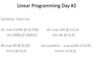
o.f.v. = $66,100 (122, 78) o.f.v. = $0 (0, 0) o.f.v. = $60,900 (174, 0) o.f.v. = $64,000 (80, 120) o.f.v. = $54,000 (0, 180) Enumerating the corner points X2 250 200 150 $15,000 100 50 0 X1 100 0 150 200 250 50
How solver views the model • Target cell - the cell in the spreadsheet that represents the objective function • Changing cells - the cells in the spreadsheet representing the decision variables • Constraint cells - the cells in the spreadsheet representing the LHS formulason the constraints • Click on Options and check “Assume Linear Model” and “Assume Non-negative”, then Solve!
Some questions • If the profit from Aqua-Spas drops to $310, what should we do? • A new product, “Portable-Spa” is considered for production. The profit is estimated to be $315/unit, and uses 1 pump, 7 hours of labor, and 14 ft. of tubing. • Should we produce it? What will be the new product mix, total profit? When we attempt to solve an LP, one of the following will occur: • Unique optimal solution • Multiple (alternate) optimal solutions • Unbounded solutions • Infeasible solution
Optimal Solution and Sensitivity Analysis • In class problem: Solved problem 1 • Formulate • Setup in Excel and solve • Interpret the solution and the sensitivity report • Formulating the business problem as an LP is the most critical and value added part. • There are many commercial solvers that can solve huge problems in minutes or even seconds. • We can use solver to gain insights to “scaled down” versions of real problems. • Group exercises: • Suggested problems: 3, 4, 5, 6