Download
1 / 95
950 likes | 1.06k Views
This study reveals the interface between speech perception and word recognition, exploring how acoustic signals are mapped onto lexical items in real-time. By examining the sensitivity to fine-grained acoustic detail and the role of sublexical units in word recognition, this work challenges the traditional notions of categorical perception. The research uncovers how continuous sensitivity to acoustic cues aids in resolving ambiguity and improving word recognition efficiency.

E N D
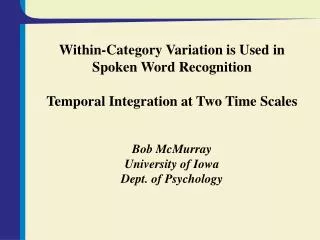
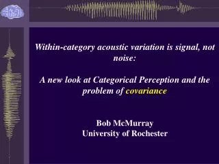
Within-category acoustic variation is signal, not noise: A new look at Categorical Perception and the problem of covariance Bob McMurray University of Rochester
Michael Tanenhaus Richard Aslin Meghan Clayards Joe Toscano Dana Subik Julie Markant David Gow* Mass General Hospital University of Rochester *Errors & Inaccuracies attributable here. Collaborators
Overview 1) Speech perception and word recognition. 2) Gradient sensitivity to acoustic detail in lexicon? 3) How might such sensitivity be used? 4) Developmental thoughts and data. 5) Conclusions
Acoustic Sublexical Units /la/ /ap/ /a/ /b/ /l/ /p/ Speech Perception: Mapping of acoustics to sublexical units. Lexicon Word Recognition: Sublexical to lexical mapping. Overview of word recognition. This work examines the interface between speech perception and spoken word recognition. To a first approximation these fields carve up the perceptual pie fairly independently. Speech Perception and Word Recognition
The interface of speech and words... Speech Perception: By the end of processing, a noisy acoustic signal is carved up into discrete units. Word Recognition: Since the early processing tosses out this variability, it can (for the most part) be ignored. Therefore: how are these units mapped onto lexical items in real-time? Combining these approaches might yield a more efficient system. Speech Perception and Word Recognition
Merging approaches Merging approaches: an example Embedded Words A purely phonemic representation creates ambiguity. shipping quietly / S I p I N kw AI t l i/ ship inquiry / S I p I N kw AI ®i/ Speech Perception and Word Recognition Q:How does the system know when to begin a new word? A coarse phonemic representation shouldyield extremely long recognition latencies (which we don’t see).
Embedded Words shipping quietly / ShIpI N kw AI t l i/ ship inquiry / Sh I ˘ ph I N kw AI ® i/ Sensitivity to fine-grained (subphonemic) detail can disambiguate the phrases. Representation of vowel length is continuous not discrete (Marslen-Wilson & Warren, 1988; Salverda, Dahan & McQueen, in press). Continuous representation of phonetic features allows probabilistic constraint satisfaction. Speech Perception and Word Recognition
We need to look at the signal… Not just embedded words... Embeddings not the only source of [phonemic] ambiguity. • Place assimilation: • Eight Babies vs. Ape Babies • If /t/ assimilated place from “Babies” this becomes ambiguous (phonemicially) Subphonemic cues could help. • Phonological Reduction: • Reduced vowels all sound like /´/ • Original vowel may leave subphonemic trace. Speech Perception and Word Recognition
A modest proposal Key properties of a combined system include: 1) Continuous sensitivity to fine-grained detail in the signal. 2) Information is retained and used to improve word recognition. Speech Perception and Word Recognition • What if the perceptual system could use fine-grained acoustic/phonetic cues to • Anticipate upcoming material • Resolve prior ambiguity • Show sensitivity to temporal organization.
100 B Discrimination % /p/ ID (%/pa/) 0 P B VOT P • Sharp identification of speech sounds on a continuum • Discrimination poor within a phonetic category Assessing continuous sensitivity Categorical Perception Speech Perception and Word Recognition Despite context dependency, system can extract phonemes (et al) remarkably discretely.
Categorical Perception • Suggests gradations in acoustic properties are discarded in favor of discrete units. • But: the strong form of CP has never been shown. Evidence against it comes from: Speech Perception and Word Recognition • Discrimination Tasks • Pisoni and Tash (1974) Pisoni & Lazarus (1974) • Carney, Widin & Viemeister (1977) • Training • Samuel (1977) Pisoni, Aslin, Perey & Hennessy (1982) • Goodness Ratings • Miller (1997) Massaro & Cohen (1983)
Categorical Perception Despite this, the notion of speech perception as discarding variability remains implicit in much of the literature. When subjects respond phonologically, performance looks categorical… But much of this work is characterized by explicit, metalinguistic tasks. Off-line measures. Non-word stimuli. Speech Perception and Word Recognition
Assessing Continuous Sensitivity These measures don’t assess lexical activation or its timecourse. But Spoken Word Recognition happens… VERY fast. Without much conscious awareness Bit-by-bit (all the information is not available at once) Need an on-line measure… Speech Perception and Word Recognition
Lexical Sensitivity to Acoustic Detail Andruski, Burton & Blumstein (1994) Misiurski, Blumstein, Rissman & Berman (in press) 3 Voiceless Tokens Peel: VOT=80 Peel1/3: VOT=53 Peel2/3: VOT=27 No difference between Peel and Peel1/3 Speech Perception and Word Recognition Fully voiceless tokens prime semantic associates better than 2/3 voiced tokens. Peel -> Banana >>>> Peel2/3 -> Banana 2/3 voiced stimuli prime competitor better than unmodified. Peach -> Sand <<<< Peach2/3 -> Sand
Lexical Sensitivity to Acoustic Detail • Andruski, Burton & Blumstein (1994) • Misiurski, Blumstein, Rissman & Berman (in press) • However: • What is the timecourse of sensitivity? • Significant effects with an ISI of 50ms. • Sometimes effects can be seen at 250ms. Speech Perception and Word Recognition
2/3 voiced stimuli were close to category boundary. • Difference between 2 items does not provide evidence for gradiency. Priming for Competitor Andruski et al (schematic) Gradient Sensitivity “Categorical” Perception 25 50 80 VOT (ms) Lexical Sensitivity to Acoustic Detail Andruski, Burton & Blumstein (1994) Misiurski, Blumstein, Rissman & Berman (in press) What is the extent of the acoustic sensitivity? Speech Perception and Word Recognition
Lexical Sensitivity to Acoustic Detail Gradiency: A monotonic relationship between lexical activation and one or more acoustic cues such that subphonemic changes in the acoustic cue result in corresponding changes in lexical activation. Gradient sensitivity to acoustic detail In short: patterns of lexical activation become a way of storing (or at least indicating) acoustic gradation. Moreover, if information is preserved in patterns of lexical activation, it must be retained long enough to be used. Need a measure sensitive to both acoustic detail and detailed temporal dynamics of lexical activation.
What kind of measure (acoustic detail)? Use speech continua—more stimulus levels yields a better picture of relationship. • KlattWorks: generate synthetic continua from natural speech. • 9-step VOT continuum (0-40 ms) • 6 pairs of words. • beach/peach bale/pale bear/pear • bump/pump bomb/palm butter/putter • 6 fillers. • Lamp Leg Lock Ladder Lip Leaf • Shark Shell Shoe Ship Sheep Shirt Gradient sensitivity to acoustic detail
How do we measure this (lexical activation)? How do we tap on-line recognition? With an on-line task: Eye-movements Subject hear spoken language and manipulate objects in a visual world. Visual world includes set of objects with interesting linguistic properties. A beach, a peach and some unrelated items. Eye-movements are monitored throughout task. Gradient sensitivity to acoustic detail
How do we measure this (lexical activation)? • Why use eye-movements and visual world paradigm? • Natural Task • Eye-movements generated very fast (within 200ms of first bit of information). • Lots of eye movements for each token. • Eye movements time-locked to speech. At any given time, an eye movement can only reflect information the subject has heard (by then). • Subjects aren’t aware of eye-movements. • Evidence that fixation probability maps onto lexical activation (Allopenna, Magnuson & Tanenhaus, 1998) Gradient sensitivity to acoustic detail
IR Headtracker Emitters Head-Tracker Cam Monitor Head 2 Eye cameras Computers connected via Ethernet Subject Computer Eyetracker Computer Head Mounted Eye Tracking Gradient sensitivity to acoustic detail
Head Mounted Eye Tracking Three cameras. One measures head position (from IR sensors on monitor) The other two record eye position. 250 Hz realtime stream of fixation coordinates. Gradient sensitivity to acoustic detail Parsed into Saccades, Fixations, Blinks, etc… Head movement compensation. Output in ~screen coordinates.
Experiment 1: Methods A moment to view the items Gradient sensitivity to acoustic detail
Experiment 1: Methods 500 ms later Gradient sensitivity to acoustic detail
Experiment 1: Methods Bear Gradient sensitivity to acoustic detail Repeat 1080 times…
1 0.9 0.8 0.7 0.6 0.5 0.4 0.3 0.2 0.1 0 0 5 10 15 20 25 30 35 40 Experiment 1: Identification Results High agreement across subjects and items for category boundary proportion /p/ Gradient sensitivity to acoustic detail B VOT (ms) P By subject:17.25 +/- 1.33ms By item: 17.24 +/- 1.24ms
Trials 1 2 3 4 5 200 ms Time Experiment 1: Fixation Analysis Gradient sensitivity to acoustic detail Target =Bear Competitor =Pear Unrelated =Lamp, Ship
0.9 0.8 VOT=0 Response= VOT=40 Response= 0.7 0.6 0.5 0.4 Fixation proportion 0.3 0.2 0.1 0 0 400 800 1200 1600 2000 0 400 800 1200 1600 Time (ms) More looks to competitor than unrelated items Experiment 1: Fixation Results Gradient sensitivity to acoustic detail
1 0.9 0.8 ID Function after filtering Actual Data 0.7 0.6 0.5 0.4 0.3 0.2 0.1 0 0 5 10 15 20 25 30 35 40 Yields a “perfect” categorization function. Experiment 1: Fixation Analysis Gradient sensitivity to acoustic detail proportion /p/ B VOT (ms) P Trials with low-frequency response excluded.
target Fixation proportion Fixation proportion time time Experiment 1: Fixation Analysis • Given that • the subject heard bear • clicked on “bear”… How often was the Subject looking at the “pear”? Categorical Results Gradient Effect Gradient sensitivity to acoustic detail target target competitor competitor competitor competitor
20 ms 25 ms 30 ms 10 ms 15 ms 35 ms 40 ms 0.16 0.14 0.12 0.1 0.08 0.06 0.04 0.02 0 0 400 800 1200 1600 0 400 800 1200 1600 2000 Experiment 1: Fixation Analysis Response= Response= VOT VOT 0 ms 5 ms Competitor Fixations Gradient sensitivity to acoustic detail Time since word onset (ms) Smaller effect on the amplitude of activation—more effect on the duration: Competitors stay active longer as VOT approaches the category boundary.
0.08 0.07 0.06 0.05 0.04 0.03 0.02 0 5 10 15 20 25 30 35 40 Area under the curve: Clear effects of VOT B: p=.026* P: p<.001*** Linear Trend B: p=.032* P: p<.001*** Experiment 1: Fixation Analysis Response= Response= Looks to Competitor Fixations Gradient sensitivity to acoustic detail Looks to Category Boundary VOT (ms)
0.08 0.07 0.06 0.05 0.04 0.03 0.02 0 5 10 15 20 25 30 35 40 Unambiguous Stimuli Only Clear effects of VOT B: p=.016* P: p<.001*** Linear Trend B: p=.012* P: p=.002** Experiment 1: Fixation Analysis Response= Response= Looks to Competitor Fixations Gradient sensitivity to acoustic detail Looks to Category Boundary VOT (ms)
0.11 0.1 0.09 Early (300-1100ms) 0.08 0.07 Late (1100-1900ms) 0.06 0.05 0.04 0.03 0.02 0.01 0 5 10 15 20 25 30 35 40 Main effect of VOT /b/: p=.015* /p/: p=.001*** Linear Trend for VOT /b/: p=.022* /p/: p=.009** No Interaction p>.1 Experiment 1: Effect of time Response= Response= Competitor Fixations Looks to Gradient sensitivity to acoustic detail Looks to Category Boundary VOT (ms)
0.11 0.1 0.09 Early (300-1100ms) 0.08 0.07 Late (1100-1900ms) 0.06 0.05 0.04 0.03 0.02 0.01 0 5 10 15 20 25 30 35 40 Unambiguous Stimuli Only Main effect of VOT /b/: p=.015* /p/: p=.001*** Linear Trend for VOT /b/: p=.022* /p/: p=.009** No Interaction p>.1 Experiment 1: Effect of time Response= Response= Competitor Fixations Looks to Gradient sensitivity to acoustic detail Looks to Category Boundary VOT (ms)
Experiment 1: Summary Subphonemic acoustic differences in VOT have gradient effect on lexical activation. • Gradient effect of VOT on looks to the competitor. • Effect holds even for unambiguous stimuli. Gradient sensitivity to acoustic detail • Effect seems to be long-lasting. Conservative Test • Filter out “incorrect” responses. • Use unambiguous stimuli only. • VOT: “Categorical” phonetic dimension.
Experiment 1: Objections You’ve probably already thought of these… 1080 is a lot of trials. Is this really tapping lexical activation or is it approaching an off-line “metalinguistic” task? Gradient sensitivity to acoustic detail Synthetic Speech—not very natural. Would effect hold up with natural tokens? VOT is not the only acoustic/phonetic dimension. Would effect hold up with other cues?
P B Sh L Bear Experiment 2: A metalinguistic task Same Stimuli Same # of trials. 16 subjects Different task: Explicit phoneme decision on initial consonant Gradient sensitivity to acoustic detail
0.1 0.09 0.08 0.07 0.06 0.05 0.04 0.03 0.02 0.01 0 0 5 10 15 20 25 30 35 40 Experiment 2: Fixation Results Response=B Looks to B Response=P Looks to B Competitor Fixations Gradient sensitivity to acoustic detail Category Boundary VOT (ms) Gradient effects using the whole range of stimuli /b/: p<.001*** ptrend<.001*** /p/: p<.001*** ptrend=.021*
0.1 0.09 0.08 0.07 0.06 0.05 0.04 0.03 0.02 0.01 0 0 5 10 15 20 25 30 35 40 Experiment 2: Fixation Results Response=B Looks to B Response=P Looks to B Competitor Fixations Gradient sensitivity to acoustic detail Category Boundary VOT (ms) Smaller effects using “unambiguous” stimuli only. /b/: p=.013* ptrend=.026* /p/: p=.297 ptrend=.075
1 0.9 0.8 0.7 0.6 0.5 0.4 An even more explicit task (Ba/Pa continuum) yielded less sensitivity in ID curve. 0.3 0.2 0.1 Exp 1: Words proportion /p/ 0 Exp 2b: BP 0 5 10 15 20 25 30 35 40 B VOT (ms) P Experiment 2: Conclusions Reduced gradient sensitivity with more explicit task. Experiment 1 results not due to subjects adopting an explicit/metalinguistic strategy. Gradient sensitivity to acoustic detail
Experiment 2: Conclusions Earlier I said: When subjects respond phonologically, performance looks categorical… This should be revised to: When subjects respond metalinguistically, performance looks categorical… Previous work overestimated categorical perception—CP is imposed on performance by the requirements of the task. Gradient sensitivity to acoustic detail
Experiment 3: Natural Stimuli Are gradient effects of VOT an artifact of synthetic speech. Same Items, Taskas Experiment 1 17 Subjects Stimuli constructed from natural tokens with progressive cross-splicing. Gradient sensitivity to acoustic detail
Experiment 3: Natural Stimuli Palm Bomb Gradient sensitivity to acoustic detail
Experiment 3: Identification Results 1 0.9 Bale 0.8 Beach 0.7 Bear 0.6 Bomb Gradient sensitivity to acoustic detail 0.5 % /p/ Response Bump 0.4 Butter 0.3 0.2 0.1 0 0 5 10 15 20 25 30 35 40 VOT Normal looking identification functions. Wider variance in category boundaries between items.
Experiment 3: Analysis of Fixations Category boundary computed from mouse-clicks for each subject, for each item. Tokens near these category boundaries excluded. Exact 5ms VOT steps could not be made with this method: VOT rounded to nearest 5ms bin. Gradient sensitivity to acoustic detail
Driven by “bale” Experiment 3: Fixation Results Response= Response= 0.09 0.08 0.07 0.06 0.05 Competitor Fixations 0.04 Gradient sensitivity to acoustic detail Looks to 0.03 Looks to 0.02 0.01 0 0 10 20 30 40 VOT (ms) Gradient effects using the whole range of stimuli /b/: p=.043* ptrend=.055 /p/: p=.001** ptrend=.007**
Experiment 3: Fixation Results Response= Response= 0.09 0.08 0.07 0.06 0.05 Competitor Fixations 0.04 Gradient sensitivity to acoustic detail Looks to 0.03 Looks to 0.02 0.01 0 0 10 20 30 40 VOT (ms) Unambiguous stimuli /b/: p<.001*** ptrend<.001*** /p/: p=.030 * ptrend=.018*
Experiment 3: Conclusions Effect not due to synthetic speech. Gradient sensitivity to VOT replicates. Gradient sensitivity to acoustic detail
Experiment 4: Other distinctions • Three R/L continua • Rake/Lake Race/Lace Ray/Lei • Six Fillers • Bees Beach Beak • Peas Peach Peak • (OK…actually another experiment) • F3 onset manipulated • Vowel held constant to reduce variability. • Same task. • Preliminary data (14 subjects). Gradient sensitivity to acoustic detail