Chapter 9 Approximating Eigenvalues
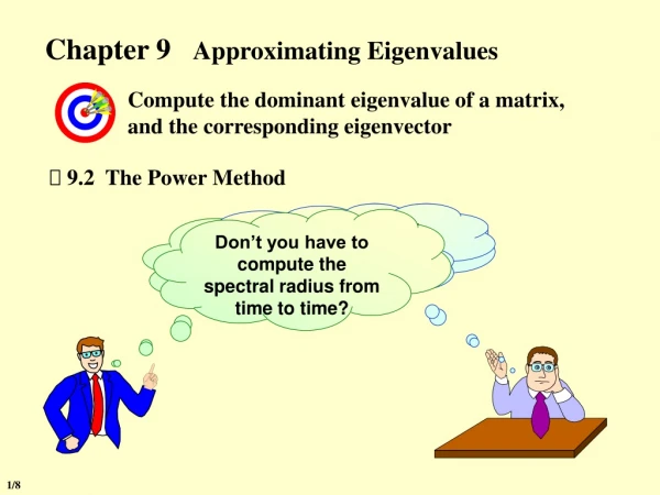
Compute the dominant eigenvalue of a matrix, and the corresponding eigenvector. Chapter 9 Approximating Eigenvalues. 9.2 The Power Method. Wait a second, what does that dominant eigenvalue mean?. Why in the earth do I want to know that?. That is the eigenvalue with the largest magnitude.

Chapter 9 Approximating Eigenvalues
E N D
Presentation Transcript
Compute the dominant eigenvalue of a matrix, and the corresponding eigenvector Chapter 9Approximating Eigenvalues 9.2 The Power Method Wait a second, what does that dominant eigenvaluemean? Why in the earth do I want to know that? That is the eigenvalue with the largest magnitude. Don’t you have to compute the spectral radius from time to time? 1/8
Chapter 9 Approximating Eigenvalues -- The Power Method Assumptions: A is an n n matrix with eigenvalues satisfying |1| > |2| … |n| 0. The eigenvalues are associated with n linearly independent eigenvectors v v Idea: Start from any and ¹ ( 0 ) ( x , v ) 0 1 This is the approximation of the eigenvector of A associated with 1 The Original Method For sufficiently large k, we have … … … 2/8
Chapter 9 Approximating Eigenvalues -- The Power Method Let . Then and Make sure that at each step to guarantee the stableness. and Normalization Algorithm: Power Method To approximate the dominant eigenvalue and an associated eigenvector of the nn matrix A given a nonzero initial vector. Input: dimension n; matrix a[ ][ ]; initial vector x0[ ]; tolerance TOL; maximum number of iterations Nmax. Output: approximate eigenvalue and approximate eigenvector (normalized) or a message of failure. 3/8
Chapter 9 Approximating Eigenvalues -- The Power Method Algorithm: Power Method (continued) Step 1 Set k = 1; Step 2 Find index such that | x0[ index ] | = || x0 || ; Step 3 Set x0[ ] = x0[ ] / x0[ index ]; /* normalize x0 */ Step 4 While ( k Nmax) do steps 5-11 Step 5 x[ ] = A x0[ ]; /* compute xk from uk1 */ Step 6 = x[ index ]; Step 7Find index such that | x[ index ] | = || x || ; Step 8 If x[ index ] == 0 then Output ( “A has the eigenvalue 0”; x0[ ] ) ; STOP. /* the matrix is singular and user should try a new x0 */ Step 9err = || x0 x / x[ index ] || ; x0[ ] = x[ ] / x[ index ]; /* compute uk */ Step 10 If (err < TOL) then Output( ; x0[ ] ) ; STOP. /* successful */ Step 11 Set k ++; Step 12 Output (Maximum number of iterations exceeded); STOP. /* unsuccessful */ 4/8
Chapter 9 Approximating Eigenvalues -- The Power Method Note: The method works for multiple eigenvalues 1 = 2 = … = r since Since we cannot guarantee 1 0 for an arbitrary initial approximation vector , the result of such iteration might not be , but be the first to satisfy . The associated eigenvalue will be m . The method fails to converge if 1 = 2 . Aitken’s 2 procedure can be used to speed the convergence. (p.563-564) 5/8
Chapter 9 Approximating Eigenvalues -- The Power Method Make | 2 / 1 |as small as possible. Idea Let B = A pI, then | IA | = | I(B+pI) | = | (p)IB | A p = B . Since , the iteration for finding the eigenvalue of B converges much faster than that of A. n 2 1 As far as the laws of mathematics refer to reality, they are not certain, and as far as they are certain, they do not refer to reality. -- Albert Einstein (1879-1955) O Rate of Convergence Assume 1 > 2 … n , and | 2 |> | n |. Determines the rate of convergence. Especially | 2 / 1 | p = ( 2+n ) / 2 How are we supposed to know where p is? 6/8
Chapter 9 Approximating Eigenvalues -- The Power Method 1 1 1 If A has eigenvalues | 1 | | 2 | … > |n |, then A1 has and they correspond to the same set of eigenvectors. > … l l l - 1 n n 1 The dominant eigenvalue of A1 The eigenvalue of A with the smallest magnitude. Idea Q: How must we compute in every step? A: Solve a linear system with A factorized. Inverse Power Method HW: Self-study Deflation Techniques on p.570-574 If we know that an eigenvalue iof A is closest to a specified number p , then for any j iwe have |i p | << |j p |. And more, if (A pI)1 exists, then the inverse power method can be used to find the dominant eigenvalue 1/(i p) of (A pI)1 with faster convergence. 7/8
Chapter 9 Approximating Eigenvalues -- The Power Method Lab 05. Approximating Eigenvalues Time Limit: 1 second; Points: 4 Approximate an eigenvalue and an associated eigenvector of a given n×n matrix A near a given value p and a nonzero vector . 8/8