
Enhancing Image Intensity Levels: Techniques and Applications
E N D
Presentation Transcript
Intensity Transformations Sections 3.1-3.3 Digital Image Processing Gonzales and Woods Irina Rabaev
Representing digital image value f(x,y) at each x, y is called intensity level or gray level
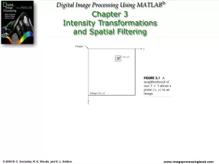
Intensity Transformations and Filters g(x,y)=T[f(x,y)] f(x,y) – input image, g(x,y) – output image T is an operator on f defined over a neighborhood of point (x,y)
Intensity Transformation • 1 x 1 is the smallest possible neighborhood. • In this case g depends only on value of f at a single point (x,y) and we call T an intensity (gray-level mapping) transformation and write s = T(r) where r and s denotes respectively the intensity of g and f at any point (x, y).
Image Negatives Denote [0, L-1] intensity levels of the image. Image negative is obtained by s= L-1-r
Log Transformations s = clog(1+r), c – const, r ≥ 0 Maps a narrow range of low intensity values in the input into a wider range of output levels. The opposite is true for higher values of input levels.
Power–Law (Gamma) transformation s = crγ, c,γ –positive constants curve the grayscale components either to brighten the intensity (when γ < 1) or darken the intensity (when γ > 1).
Contrast stretching Contrast stretching is a process that expands the range of intensity levels in a image so that it spans the full intensity range of the recording medium or display device. Contrast-stretching transformations increase the contrast between the darks and the lights
Intensity-level slicing Highlighting a specific range of gray levels in an image
Histogram processing The histogram of a digital image with gray levels in the range [0, L-1] is a discrete function h(rk)=nk, where rk is the kth gray level and nk is the number of pixels in the image having gray level rk. It is common practice to normalize a histogram by dividing each of its values by the total number of pixels in the image, denoted by the product MN. Thus, a normalized histogram is given by h(rk)=nk/MN The sum of all components of a normalized histogram is equal to 1.
Histogram Equalization • Histogram equalization can be used to improve the visual appearance of an image. • Histogram equalization automatically determines a transformation function that produce and output image that has a near uniform histogram
Histogram Equalization • Let rk, k[0..L-1] be intensity levels and let p(rk) be its normalized histogram function. • The intensity transformation function for histogram equalization is
Histogram Equalization - Example • Let f be an image with size 64x64 pixels and L=8 and let f has the intensity distribution as shown in the table round the values to the nearest integer
Local histogram Processing Define a neighborhood and move its center from pixel to pixel. At each location, the histogram of the points in the neighborhood is computed and histogram equalization transformation is obtained.
Using Histogram Statistics for Image Enhancement Denote: ri – intencity value in the range [0, L-1], p(i) - histogram component corresponding to value ri . The intensity variance:
Using Histogram Statistics for Image Enhancement Let (x, y) be the coordinates of a pixel in an image, and let Sxydenote a neighborhood (subimage) of specified size, centered at (x, y). The mean value of the pixels in this neighborhood is given by where is the histogram of the pixels in region Sxy. The variance of the pixels in the neighborhood is given by
Using Histogram Statistics for Image Enhancement Tungsten filament