Image Processing and Transformations: A Guide to Histogram Equalization and Intensity Changes
This chapter explores the spatial domain methods in image processing with a focus on intensity transformations. Key techniques such as identity transformation, negative image processing, contrast stretching, and histogram equalization are discussed in detail. The principles of image histograms, probability distributions, and random variables are also clarified, leading to advanced methods like histogram specification. By understanding these transformations, we can effectively enhance image quality, highlighting specific details or compressing uninformed ranges.

Image Processing and Transformations: A Guide to Histogram Equalization and Intensity Changes
E N D
Presentation Transcript
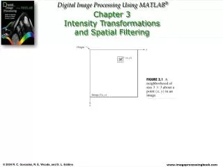
Intensity Transformations (Chapter 3) CS474/674 – Prof. Bebis
Spatial Domain Methods f(x,y) g(x,y) Point Processing g(x,y) f(x,y) Area/Mask Processing
Point Processing Transformations • Convert a given pixel value to a new pixel value based on some predefined function.
Negative Image • O(r,c) = 255-I(r,c)
Contrast Stretching or Compression • Stretch gray-level ranges where we desire more information (slope > 1). • Compress gray-level ranges that are of little interest (0 < slope < 1).
Thresholding • Special case of contrast compression
Intensity Level Slicing • Highlight specific ranges of gray-levels only. Same as double thresholding!
Bit-level Slicing • Highlighting the contribution made by a specific bit. • For pgm images, each pixel is represented by 8 bits. • Each bit-plane is a binary image
Logarithmic transformation • Enhance details in the darker regions of an image at the expense of detail in brighter regions. compress stretch
Exponential transformation • Reverse effect of that obtained using logarithmic mapping. stretch compress
Histogram Equalization • A fully automatic gray-level stretching technique. • Need to talk about image histograms first ...
Image Histograms • An image histogram is a plot of the gray-level frequencies (i.e., the number of pixels in the image that have that gray level).
Image Histograms (cont’d) • Divide frequencies by total number of pixels to represent as probabilities.
Properties of Image Histograms • Histograms clustered at the low end correspond to dark images. • Histograms clustered at the high end correspond to bright images.
Properties of Image Histograms (cont’d) • Histograms with small spread correspond to low contrastimages (i.e., mostly dark, mostly bright, or mostly gray). • Histograms with wide spread correspond to high contrastimages.
Properties of Image Histograms (cont’d) High contrast Low contrast
Histogram Equalization • The main idea is to redistribute the gray-level values uniformly.
Histogram Equalization (cont’d) • In practice, the equalized histogram might not be completely flat.
Probability - Definitions • Random experiment: an experiment whose result is not certain in advance (e.g., throwing a die) • Outcome: the result of a random experiment • Sample space: the set of all possible outcomes (e.g., {1,2,3,4,5,6}) • Event: a subset of the sample space (e.g., obtain an odd number in the experiment of throwing a die = {1,3,5})
Random Variables - Review • A function that assigns a real number to random experiment outcomes (i.e., helps to reduce space of possible outcomes) X(j) X: # of heads
Random Variables - Example • Consider the experiment of throwing a pair of dice • Define the r.v. X=“sum of dice” • X=x corresponds to the event
Probability density function • The probability density function(pdf) is a real-valued function fX(x) describing the density of probability at each point in the sample space. • In the discrete case, this is just a histogram! Gaussian
Gaussian fX(a)da non-decreasing Probability distribution function • The integral of fX(x) defines the probability distribution functionFX(x) (i.e., cumulative probability) • In the discrete case, simply take the sum: fX(x) FX(x)
Uniform Distribution FX(x) fX(x) B_Parvin@lbl.gov
Random Variable Transformations • Suppose Y=T(X) • e.g., Y=X+1 • If we know fX(x), can we find fY(y)? • Yes - it can be shown that:
Transformations of r.v. - Example μ=0, σ=1 0 μ=1, σ=1
Special transformation! Proof:
Histogram Equalization (cont’d) The intensity levels can be viewed as a random variable in [0,1] ps(s) pr(r)
Histogram Equalization (cont’d) For PGM images: L=256 (graylevels) k=0,1,2, …, L-1 (possible graylevels) rk=k/(L-1) (normalized graylevel in [0, 1])
Histogram Equalization (cont’d) then, de-normalize: sk x (L-1)
Histogram Equalization Example 3 bit 64 x 64 image input histogram equalized histogram
Histogram Equalization Examples original images and histograms equalized images and histograms
only desired histogram is known fR(r) fZ(z) fR(a)da fZ(a)da Histogram Specification (Matching) • Histogram equalization yields a uniform pdf only. • What if we want to obtain a histogram other than uniform? so, Q(r)=G-1(T(r))
Histogram Specification (cont’d) • fS(s) and fV(v) are uniform • G(z) can be computed by specifying fZ(z) but I2 and I’2 are unknown! • z=G-1(v) requires that v is a r.v. with uniform pdf • IDEA: use z=G-1(s) instead of z=G-1(v) • s is a r.v. with uniform pdf • The desired transformation is z=G-1(T(r)) fR(a)da fz(a)da
Histogram Specification (cont’d) • Comments • We do not need to apply T( ) and G-1( ) separately! • Combine them: Q=G-1T, thus, z=Q(r) • Histogram specification assumes that we know G-1 (not always easy to find). • G( ) must be in [0,1] and must be non-decreasing. z=G-1(T(r))=Q(r)
Histogram Specification Example 3 bit 64 x 64 image input histogram specified histogram actual histogram
Histogram Specification (cont’d) • Histogram specification might yield superior results than histogram equalization. results of histogram equalization
Histogram Specification (cont’d) results of histogram specification G(z) G-1(z)
Local Histogram Processing • Histogram equalization/specification are global methods. • The intensity transformation is computed using pixels from the entire image. • Global transformations are not appropriate for enhancing little details in an image. • The number of pixels in these areas might be very small, contributing very little to the computation of the transformation.
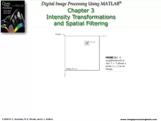
Local Histogram Processing Idea: Define a transformation function based on the intensity distribution in a neighborhood of every pixel in the image!
Local Histogram Processing (cont’d) 1. Define a neighborhood and move its center from pixel to pixel. 2. At each location, the histogram of the points in the neighborhood is computed. Obtain histogram equalization or histogram specification transformation. 3. Map the intensity of the pixel centered in the neighborhood. 4. Move to the next location and repeat the procedure.
Local Histogram Processing: Example local histogram equalization 3 x 3 neighborhood global histogram equalization
Histogram Statistics Mean (average intensity) n-th moment around mean Variance (2nd moment)
Example: Comparison of Standard Deviation Values σ is useful for estimating image contrast!
Using Histogram Statistics for Image Enhancement • Useful when parts of the image might contain hidden features. Task: enhance dark areas without changing bright areas. Idea: Find dark, low contrast areas using local statistics.