3.5 Random Vibrations
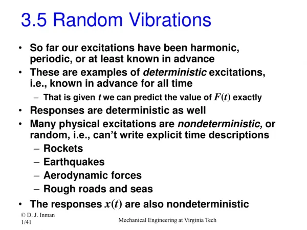
3.5 Random Vibrations. So far our excitations have been harmonic, periodic, or at least known in advance These are examples of deterministic excitations, i.e., known in advance for all time That is given t we can predict the value of F ( t ) exactly Responses are deterministic as well

3.5 Random Vibrations
E N D
Presentation Transcript
3.5 Random Vibrations So far our excitations have been harmonic, periodic, or at least known in advance These are examples of deterministic excitations, i.e., known in advance for all time That is given t we can predict the value of F(t) exactly Responses are deterministic as well Many physical excitations are nondeterministic, or random, i.e., can’t write explicit time descriptions Rockets Earthquakes Aerodynamic forces Rough roads and seas The responses x(t) are also nondeterministic Mechanical Engineering at Virginia Tech
Random Vibrations • Stationary signals are those whose statistical properties do not vary over time • Functions are described in terms of probabilities • Mean values* • Standard deviations • Random outputs related to random input via system transfer function *ie given t we do not know x(t) exactly, but rather we only know statistical properties of the response such as the average value Mechanical Engineering at Virginia Tech
Autocorrelation function and power spectral density The autocorrelation function describes how a signal is changing in time or how correlated the signal is at two different points in time. The Power Spectral Density describes the power in a signal as a function of frequency and is the Fourier transform of the autocorrelation function. FFT is a new way for calculating Fourier Transforms Mechanical Engineering at Virginia Tech
Examples of signals HARMONIC RANDOM T Signal A Arms x(t) time time x(t) -A T A2rms A2/2 Autocorrelation t time shift t time shift Rxx(t) Rxx(t) -A2/2 Power Spectral Density Sxx(w) Sxx(w) Frequency (Hz) Frequency (Hz) 1/T Mechanical Engineering at Virginia Tech
More Definitions Average: Mean-square: rms: Mechanical Engineering at Virginia Tech
Expected Value (or ensemble average) The expected value = The Probability Density Function, p(x), is the probability that x lies in a given interval (e.g. Gaussian Distribution) The expected value is also given by Mechanical Engineering at Virginia Tech
Recall the Basic Relationships for Transforms: Recall for SDOF: And the Fourier Transform of h(t)isH(w) Mechanical Engineering at Virginia Tech
What can you predict? The response of SDOF with f(t) as input: Deterministic Input: Random Input: In a Lab, the PSD function of a random input and the output can be measured simply in one experiment. So the FRF can be computed as their ratio by a single test, instead of performing several tests at various constant frequencies. Here we get an exact time record of the output given an exact record of the input. Here we get an expected value of the output given a statistical record of the input. Mechanical Engineering at Virginia Tech
Example 3.5.1 PSD Calculation The corresponding frequency response function is: From equation (3.62) the PSD of the response becomes: Mechanical Engineering at Virginia Tech
Example 3.5.2 Mean Square Calculation Consider the system of Example 3.5.1 and compute: Here the evaluation of the integral is from a tabulated value See equation (3.70). Mechanical Engineering at Virginia Tech
Section 3.6 Shock Spectrum Arbitrary forms of shock are probable (earthquakes, …) The spectrum of a given shock is a plot of the maximum response quantity (x) against the ratio of the forcing characteristic (such as rise time) to the natural period. Maximum response gives maximum stress. Mechanical Engineering at Virginia Tech
Using the convolution equation as a tool, compute the maximum value of the response Recall the impulse response function undamped system: Such integrals usually have to be computed numerically Mechanical Engineering at Virginia Tech
Example 3.6.1 Compute the response spectrum for gradual application of a constant force F0. Assume zero initial conditions t1=infinity, means static loading F(t) F0 t t1 The characteristic time of the input Mechanical Engineering at Virginia Tech
Split the solution into two parts and use the convolution integral (3.75) For x2 apply time shift t1 (3.76) (3.77) Mechanical Engineering at Virginia Tech
Next find the maximum value of this response To get max response, differentiate x(t). In the case of a harmonic input (Chapter 2) we computed this by looking at the coefficient of the steady state response, giving rise to the Magnitude plots of figures 2.7, 2.8, 2.13. Need to look at two cases 1) t < t1 and 2) t>t1 For case 2) solve: (what about case 1? Its max is Xstatic) Mechanical Engineering at Virginia Tech
Solve for t at xmax, denoted tp Mechanical Engineering at Virginia Tech
From the triangle: Minus sq root taken as + gives a negative magnitude Substitute into x(tp) to get nondimensionalXmax : 1st term is static, 2nd is dynamic. Plot versus: Input characteristic time System period Mechanical Engineering at Virginia Tech
Response Spectrum • Indicates how normalized max output • changes as the input pulse width increases. • Very much like a magnitude plot. • Shows very small t1 can increase • the response significantly: impact, rather than • smooth force application • The larger the rise time, the smaller the peaks • The maximum displacement is minimized if • rise time is a multiple of natural period • Design by MiniMax idea Mechanical Engineering at Virginia Tech
Comparison between impulse and harmonic inputs Impulse Input Transient Output Max amplitude versus normalized pulse “frequency” Harmonic Input Harmonic Output Max amplitude versus normalized driving frequency Mechanical Engineering at Virginia Tech
Review of The Procedure for Shock Spectrum • Find x(t) using convolution integral • Compute its time derivative • Set it equal to zero • Find the corresponding time • Evaluate the max possible value of x (be careful about points where the function does not have derivative!!) • Plot it for different input shocks Mechanical Engineering at Virginia Tech
3.7 Measurement via Transfer Functions • Apply a sinusoidal input and measure the response • Do this at small frequency steps • The ratio of the Laplace transform of these to signals then gives and experiment transfer function of the system Mechanical Engineering at Virginia Tech
Several different signals can be measured and these are named Mechanical Engineering at Virginia Tech
The magnitude of the compliance transfer function yields information about the systems parameters Mechanical Engineering at Virginia Tech
3.8 Stability Stability is defined for the solution of free response case: Stable: Asymptotically Stable: Unstable: if it is not stable or asymptotically stable Mechanical Engineering at Virginia Tech
Recall these stability definitions for the free response Stable Asymptotically Stable Divergent instability Flutter instability Mechanical Engineering at Virginia Tech
Stability for the forced response: • Bounded Input-Bounded Output Stable • x(t) bounded for ANY bounded F(t) • Lagrange Stable with respect to F(t) • If x(t) is bounded for THE given F(t) Mechanical Engineering at Virginia Tech
Relationship between stability of the homogeneous system and the force response • If xhomo is Asymptotically stable then the forced response is BIBO stable (Bounded input, bounded output) • If xhomo is Stable then the forced response MAY be Lagrange Stable or Unstable Mechanical Engineering at Virginia Tech
Stability for Harmonic Excitations The solution to: is: As long as n is not equal to this is Lagrange Stable, if the frequencies are equal it is Unstable Mechanical Engineering at Virginia Tech
For underdamped systems: Add homogeneous and particular to get total solution: Bounded Input-Bounded Output Stable Mechanical Engineering at Virginia Tech
Example 3.8.1 • The system is thus • Lagrange stable. • Physically this tells us • the spring must be large • enough to overcome • gravity Mechanical Engineering at Virginia Tech
3.9 Numerical Simulation of the response • As before in Section 2.8 write equations of motion as state space equations • The Euler integration is just Mechanical Engineering at Virginia Tech
F(t) F0 m t0 Example 3.9.1 with delay Let the input force be a step function a t=t0 x(t) F0=30N k=1000N/m z=0.1 wn=3.16 t0=2 k c Mechanical Engineering at Virginia Tech
Example 3.9.1 Analytical versus numerical • Response to step input • clear all • %% Analytical solution (example 3.2.1) • Fo=30; k=1000; wn=3.16; zeta=0.1; to=0; • theta=atan(zeta/(1-zeta^2)); • wd=wn*sqrt(1-zeta^2); • t=0:0.01:12; • Heaviside=stepfun(t,to);% define Heaviside Step function for 0<t<12 • xt = (Fo/k - Fo/(k*sqrt(1-zeta^2)) * exp(-zeta*wn*(t-to)) * • cos (wd*(t-to)- theta))*Heaviside(t-to); • plot(t,xt); hold on • %% Numerical Solution • xo=[0; 0]; • ts=[0 12]; • [t,x]=ode45('f',ts,xo); • plot(t,x(:,1),'r'); hold off • %--------------------------------------------- • function v=f(t,x) • Fo=30; k=1000; wn=3.16; zeta=0.1; to=0; m=k/wn^2; • v=[x(2); x(2).*-2*zeta*wn + x(1).*-wn^2 + Fo/m*stepfun(t,to)]; Mechanical Engineering at Virginia Tech
0.06 0.05 0.04 Displacement (x) 0.03 0.02 0.01 0 0 2 4 6 8 10 12 Time (s) Matlab Code x0=[0;0]; ts=[0 12]; [t,x]=ode45('funct',ts,x0); plot(t,x(:,1)) function v=funct(t,x) F0=30; k=1000; wn=3.16; z=0.1; t0=2; m=k/(wn^2); v=[x(2); x(2).*-2*z*wn+x(1).*-wn^2+F0/m*stepfun(t,t0)]; Mechanical Engineering at Virginia Tech
Numerical solution of Problem 3.19 %problem 3.19 m=1000; E=3.8e9; A=0.03; L=2; k=E*A/L; t0=0.2; F0=100; global F0 k m t0 %numerical solution x0=[0;0]; ts=[0 0.5]; [t,x]=ode45('f_3_19',ts,x0); plot(t,x(:,1)) F(t) function v=f_3_19(t,x) global F0 k m t0 A=x(2); F=(((1-t./t0).*stepfun(t,0))-((1-t./t0).*stepfun(t,t0)))*F0/m; B=(-k/m)*x(1)+F; v=[A; B]; Mechanical Engineering at Virginia Tech
P3.19 Variations in correct direction Displacement Mechanical Engineering at Virginia Tech
3.9 Nonlinear Response Properties Euler integration formula: Nonlinear term Analytical solutions not available so we must interrogate the numerical solution Mechanical Engineering at Virginia Tech
Example 3.10 cubic spring subject to pulse input The state space form is: Mechanical Engineering at Virginia Tech
Nature of Response Red (solid) is nonlinear response. Blue (dashed) is linear response Is there any justification? Yes, hardening nonlinear spring. The first part is due to IC. Mechanical Engineering at Virginia Tech
Matlab Code clear all xo=[0.01; 1]; ts=[0 8]; [t,x]=ode45('f',ts,xo); plot(t,x(:,1)); hold on % The response of nonlinear system [t,x]=ode45('f1',ts,xo); plot(t,x(:,1),'--'); hold off % The response of linear system %--------------------------------------------- function v=f(t,x) m=100; k=2000; c=20; wn=sqrt(k/m); zeta=c/2/sqrt(m*k); Fo=1500; alpha=3; t1=1.5; t2=5; v=[x(2); x(2).*-2*zeta*wn + x(1).*-wn^2 - x(1)^3.*alpha+ Fo/m*(stepfun(t,t1)-stepfun(t,t2))]; %--------------------------------------------- function v=f1(t,x) m=100; k=2000; c=20; wn=sqrt(k/m); zeta=c/2/sqrt(m*k); Fo=1500; alpha=0; t1=1; t2=5; v=[x(2); x(2).*-2*zeta*wn + x(1).*-wn^2 - x(1)^3.*alpha+ Fo/m*(stepfun(t,t1)-stepfun(t,t2))]; Mechanical Engineering at Virginia Tech
What good is this ability? • Investigate pulse width • Investigate parameter changes • Investigate effect of initial conditions • Design and Prediction Because there are not many closedf form solutions, or magnitude expressions design must be done by numerical simulation Mechanical Engineering at Virginia Tech