Amortized Supersampling
Amortized Supersampling. Lei Yang H , Diego Nehab M , Pedro V. Sander H , Pitchaya Sitthi-amorn V , Jason Lawrence V , Hugues Hoppe M. Dec. 18, 2009, Pacifico Yokohama, Japan. Outline. Problem Amortized supersampling – basic approach Challenge - the resampling blur

Amortized Supersampling
E N D
Presentation Transcript
Amortized Supersampling Lei Yang H, Diego NehabM, Pedro V. Sander H, PitchayaSitthi-amornV, Jason Lawrence V, Hugues Hoppe M Dec. 18, 2009, Pacifico Yokohama, Japan
Outline • Problem • Amortized supersampling – basic approach • Challenge - the resampling blur • Our algorithm • Results and conclusion
Problem • Shading signals not band-limited • Procedural materials • Complex shading functions • Band-limited version (analytically antialiased) • Ad-hoc • Difficult to obtain
Problem • Supersampling • General antialiasing solution • Compute a Monte-Carlo integral • Can be prohibitively expensive
Accelerating Supersampling • Shading functions usually vary slowly over time • Reuse samples from previous frames • Reprojection • Generate only one sample every frame …… Frame 1 Frame 2 Frame 3 Frame t
Amortized Supersampling • Cannot afford to store all the samples from history • Keep only a running accumulated result • Update it every frame using exponential smoothing = Frame t Frame 1 ~ t-1 Frame t-1
Reverse Reprojection [Nehab07, Scherzer07] • Compute previous location πt-1(p) of point p • A bilinear texture fetch for the previous value • Check depth for occlusion changes p πt-1(p)
Effect of the smoothing factor α • Larger α: less history, more aliasing/noise • Smaller α: less fresh value, more smoothing • Equal weight of samples: (1 – α) · + (α) · → Frame t Frame t-1
An artifact of recursive reprojection • Severe blur due to repeated bilinear interpolation Recursivereprojection Ground truth
Factors of the blur • Fractional pixel velocity v = (vx, vy) • Exponential smoothing factor α v =(0.5, 0.5) …… Frame t-3 Frame t-2 Frame t-1 Frame t (1- α)3 (1- α)2 (1- α) …… Frame t-3 Frame t-2 Frame t-1 Frame t
The amount of blur • The expected blur variance is (derivation in the appendix) • Approaches for reducing the blur: • Increase resolution of the history buffer • Avoid bilinear resampling whenever possible • Limit α when needed
(1) Increase resolution • Option 1:Keep a history buffer at high resolution (2x2) • Have to update it every frame • Option 2:Keep 4 subpixel buffers at normal resolution • Only update one of them each frame Subpixel buffers High-resolution buffer
(2) Avoid bilinear sampling • Reconstructing from subpixel buffers • Forward reproject the samples from 4 subpixel buffers to the current subpixel quadrant • Weight them using a tent function • GPU approximation/acceleration
(3) Limiting blur via bounding α • Derive a relationship between • Blur variance σ 2 • Motion velocity v and α • Analytic relationship is not attainable • Numerical simulation and tabulate • Bound α for limiting σ2 no larger than τb
Adaptive evaluation • Newly disoccluded pixels are prone to aliasing • Additional shading for subpixels that fail in reconstruction
Accounting for signal changes • Detect fast signal change • React by more aggressive update • Estimate residual ε between: • Current sample st(aliased/noisy) • History estimate ft • Blur the residual estimate to remove aliasing/noise • Bound α for limiting ε no larger than τε
Conclusion • A real-time scheme for amortizing supersampling costs • Quality comparable to 4x4 stratified supersampling • Speed is 5x-10x of 4x4 supersampling • A single rendering pass